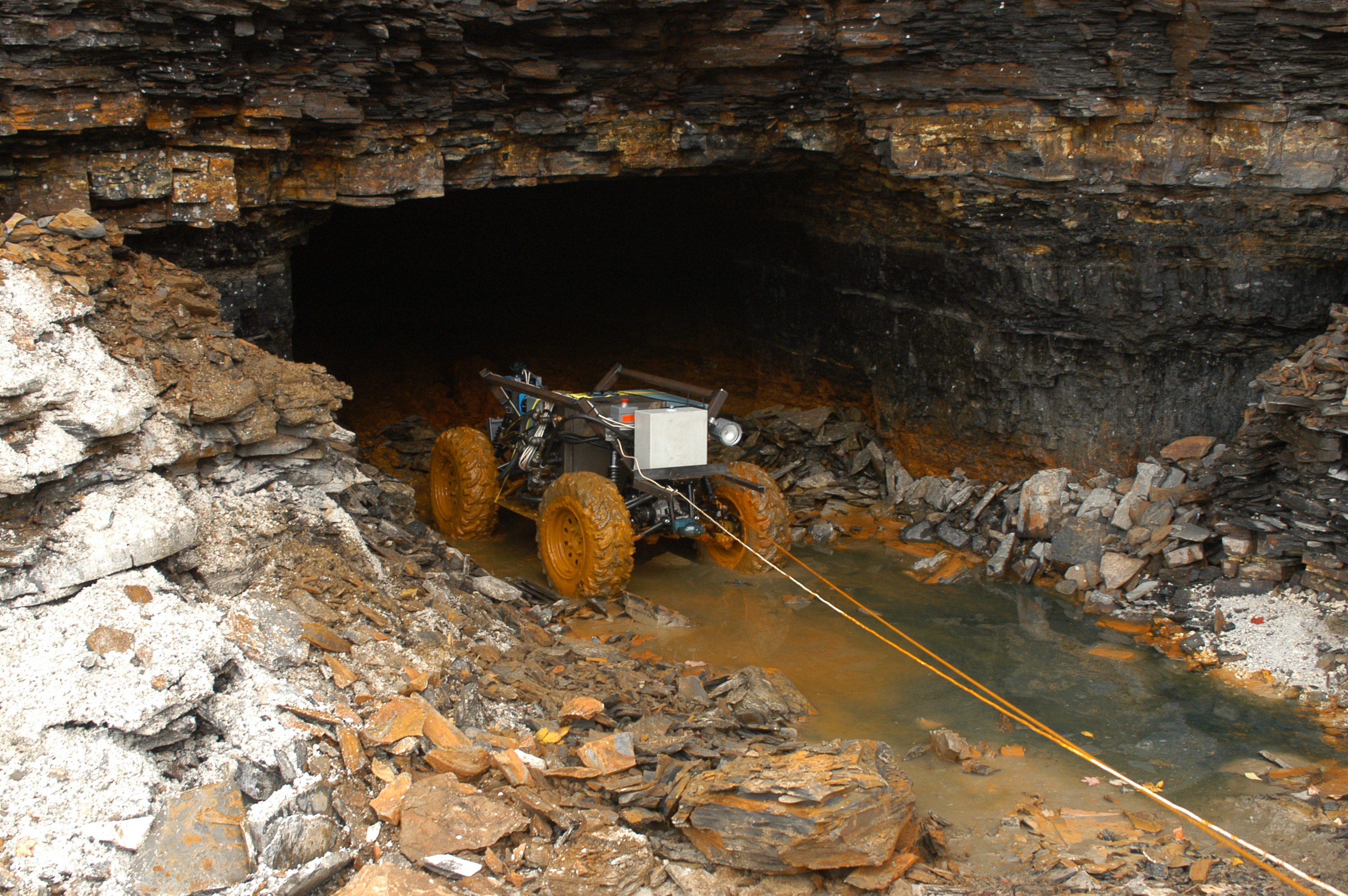
In year 2003 the team of scientists from the Carnegie Mellon university has created a mobile robot called Groundhog, which could explore and create the map of an abandoned coal mine. The rover explored tunnels, which were too toxic for people to enter and where oxygen levels were too low for humans to remain concious. The task was not easy: navigate in the environment, which the robot has not seen before, and simultaneously discover and create a map of those unknown tunnels.

The groundhog robot enters the abandoned coal mine. (source: www.cs.cmu.edu)

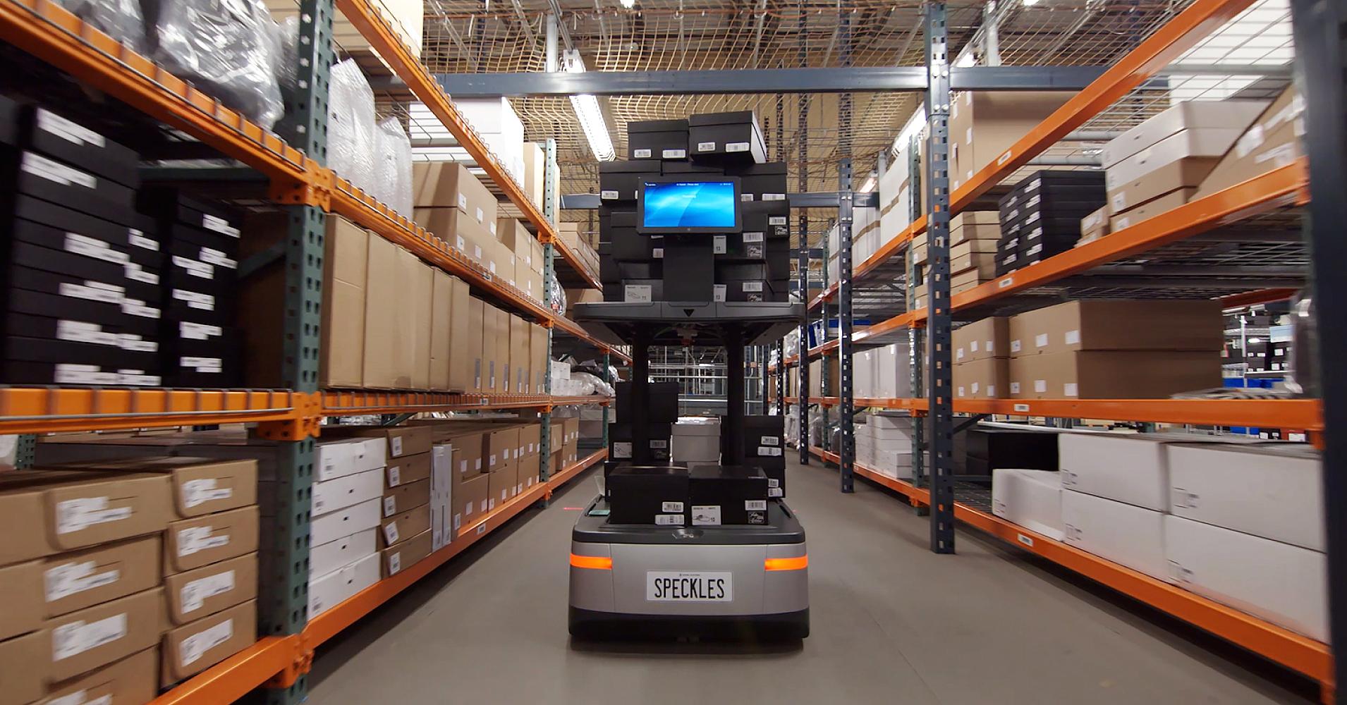
Fifteen years later, the problem of constructing a map of an unknown environment, while keeping track of agent’s location within it (the so called SLAM task- Simultaneous Localization And Mapping), is still being scrutinized by the researchers. This notion is not only used in the fields of self-driving cars or rovers, but is also present in case of domestic robots such as iRobot’s Roomba. In the year 2017 Amazon has doubled the number of its robotic fleet. So far, the robo-workers are there to move packages through the gigantic warehouses, but it is only a matter of time until advanced robots will work hand in hand with actual people, performing more complicated tasks. This shows that given current state of the technology, the ability for robots to understand their position in the environment is indispensable.

Chuck, a robotic warehouse assistant. Perhaps in the near future warehouses will be operated only by sophisticated robots... (source: www.cnbc.com)

The goal of this tutorial is to tackle a simple case of mobile robot localization problem using Hidden Markov Models. Let’s use an example of a mobile robot in a warehouse. The agent is randomly placed in an environment and we, its supervisors, cannot observe what happens in the room. The only information we receive are the sensor readings from the robot.

Table of Contents

• Case formulation
  • Environment
  • Sensors
  • Hidden Markov Models
• Let’s solve the problem!
  • Transition model
  • Initial state
  • Sensor model
  • Results
  • Alternative possible solutions
  • The code in Python

Case formulation

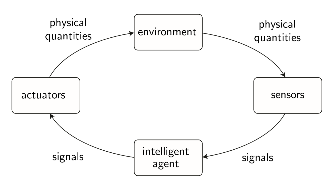
“An agent is anything that can be viewed as perceiving its environment through sensors and acting upon that environment through effectors”

Source: Artificial Intelligence: A Modern Approach (S. Russell and P. Novig)

To fully define a case we need to specify two pieces of information:

• environment (the warehouse),
• sensor model (how the robot perceives the environment)

Environment

Figure 1: Environment of the robot

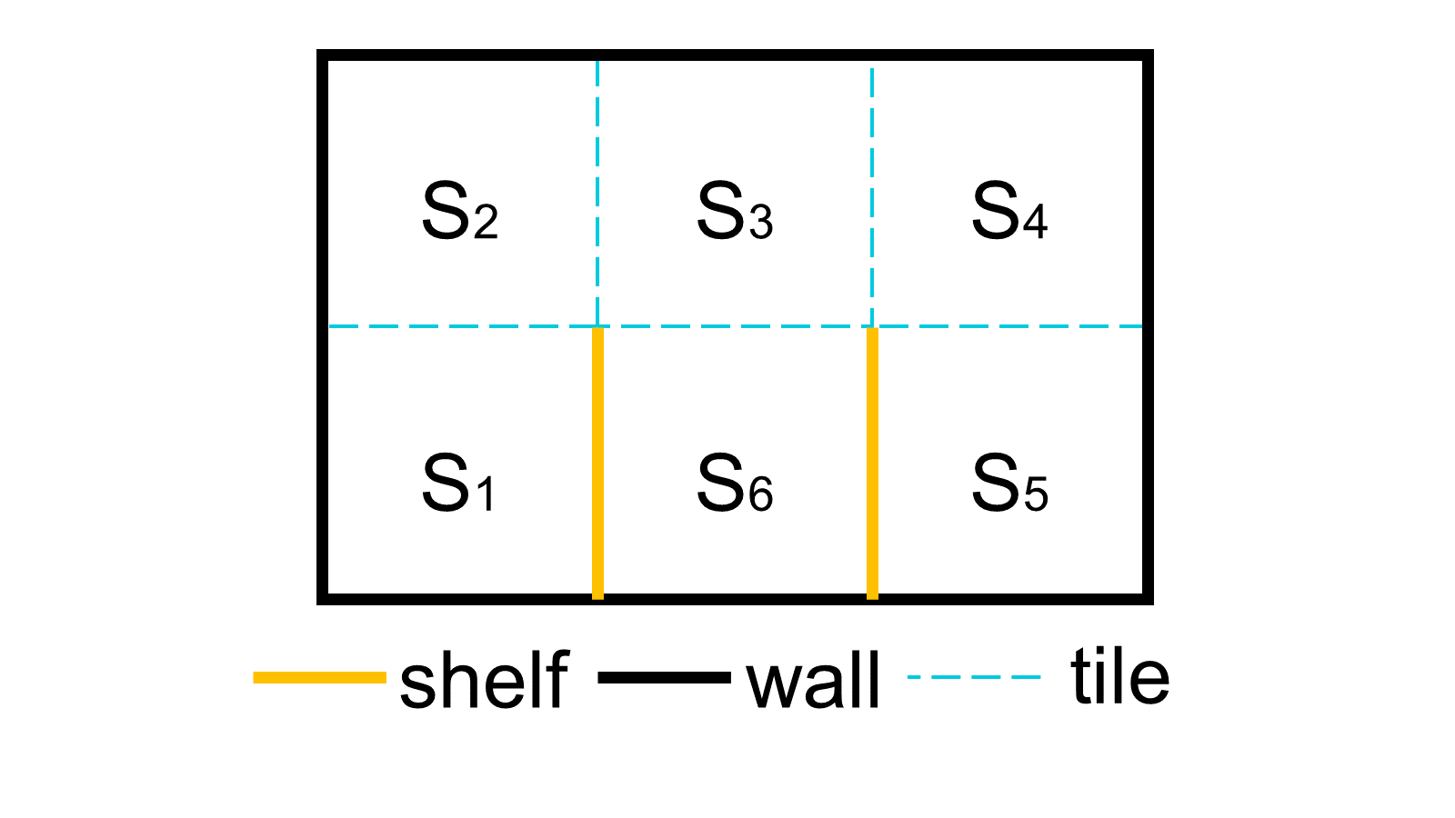
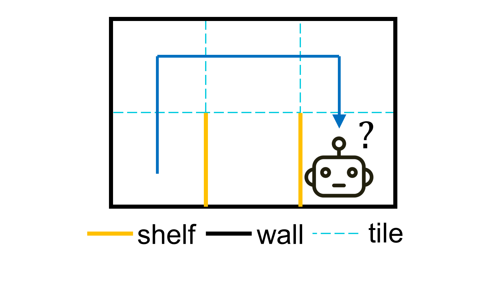
The agent can move within an area of 6 square tiles. In the mini-warehouse there is one shelf located between tiles \(S_1\) and \(S_6\) and a second shelf between \(S_6\) and \(S_5\). In the technical jargon one may say, that the environment of the agent consists of six descrete states. The time is also descrete. At each subsequent time step the robot is programmed to change its position with a probability of 80% and moves randomly to a different neighboring tile. As soon as the robot makes a move, we receive four readings from the sensing system.

Figure 2: Probabilistic graphical model

Sensors

Just as we humans can localizate ourselves using senses, robots use sensors. Our agent is equipped with the sensing system composed of a compass and a proximity sensor, which detects obstacles in four directions: north, south, east and west. The sensor values are conditionally independent given the position of the robot. Moreover, the device is not perfect, the sensor has an error rate of e=25%.

Hidden Markov Models

The Hidden Markov Model (HMM) is a simple way to model sequential data. There exists some state \(X\) that changes over time. It is assumed that this state at time t depends only on previous state in time t-1 and not on the events that occurred before ( why known as Markov property). We wish to estimate this state \(X\). Unfortunately, we cannot directly observe it, the state is not directly visible (hidden). However, we can observe a piece of information correlated with the state, the evidence \(E\), which helps us to estimate \(X\).

Figure 3: Temporal evolution of a hidden Markov model

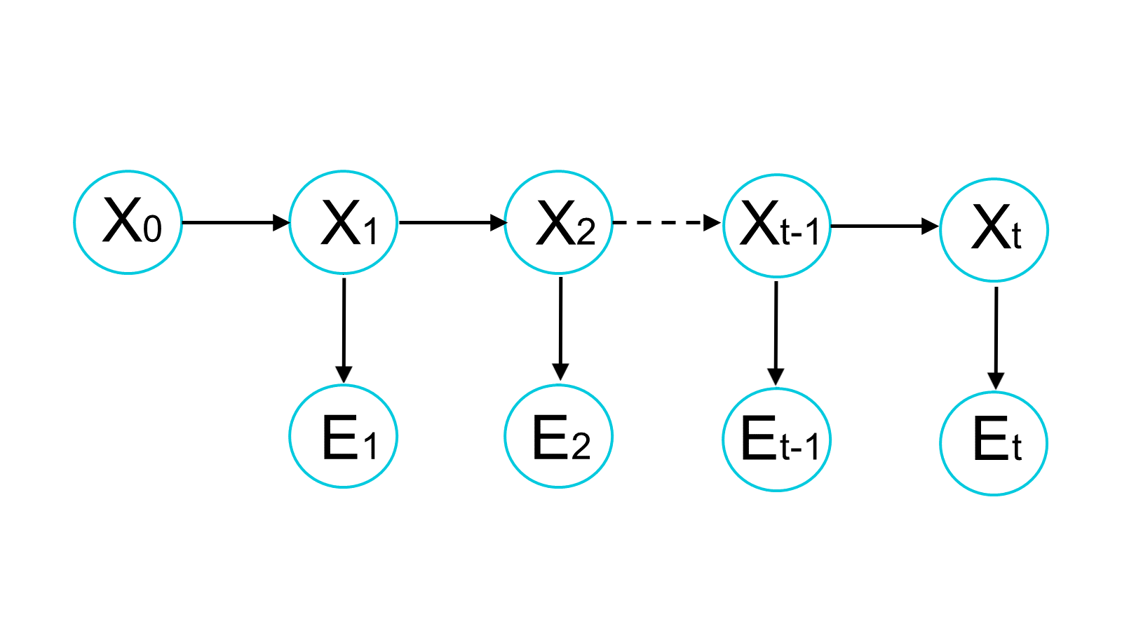
Our model consists of hidden states \(X_0,X_1,X_2,..., X_{t-2}, X_{t-1},X_t\) (the unknown location of a robot in time) and known pieces of evidence \(E_1, E_2, ..., E_{t-2},E_{t-1},E_t\) (the subsequent readings from the sensor).

There are two tools which we use to localize the robot:

• filtering- estimation of the state in time \(X_t\), knowing the state \(X_{t-1}\) and evidence \(E_{t}\).

• prediction- filtering without evidence. We make a guess about the \(X_t\)knowing only state \(X_{t-1}\).

where:

• \({f_{1:t}}\) current probability vector in time t
• \({f_{1:t-1}}\) previous probability vector in time t-1
• \({\alpha}\) normalization constant
• \({O_t}\) observation matrix for the evidence in time t
• \({T}\) transition matrix

Let’s solve the problem!

Transition model

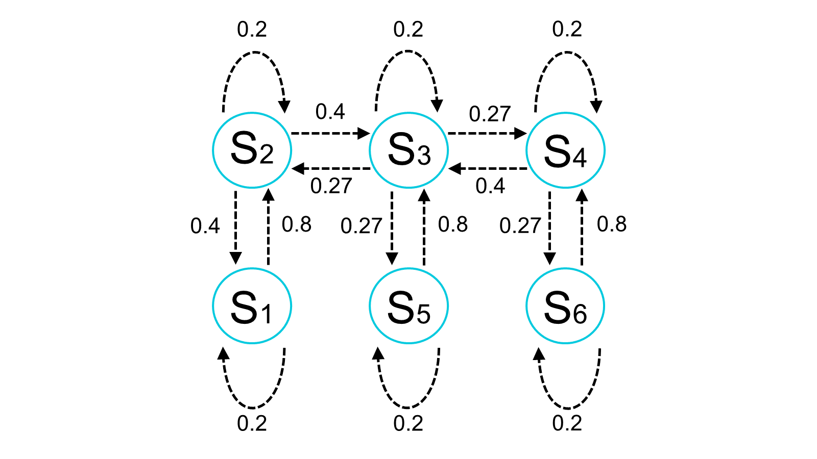
The transition model is the probability of a transition from state i to state j . This can be mathematically expressed as:

What is the meaning of this formula? Knowing that at time t-1 the agent was in state i, it gives us the probability of the agent being in state j in the current time t . To make it clearer, let’s give an example.

The robot changes his position from tile 1 to tile 2. This means the transition from \(S_1\) to \(S_2\) . We see from figure 2, that the probability of this transition equals 80%.

This solution is only one of many transitions possible for the robot in our environment. The domain of the state variable \(X_t\) is a set of all the possible tiles in the environment: \(<{S_1,S_2,S_3,S_4,S_5,S_6}>\) . Hence, the full transition matrix, which contains all the possible transitions from state i to state j, will have 6x6=36 entries.

Initial state

To make the problem more interesting, let’s assume that we do not know the initial position of the robot. The logical approach is to assume a uniform probability distribution over all tiles of the grid. Since our environment consists of 6 states, we can say that for any of those 6 states (let’s call this hypothetical state i ), the probability that the agent starts its adventure in square i is:

We can express this probability for all six states using vector notation:

Sensor model

Sensor model consists out of evidence, which allows to make inference about the agent’s position in the environment. In the first time step robot detects a wall in directions: south, west and east. How can we express this information in the mathematical notation? We want to find the answer to the question: given that we are in state i, what is the probability that the sensor returns reading \({E=j}\)? That is:

where e is an error rate of a sensor and d is the discrepancy- a number of signals that are different- between the true values for tile i and the actual reading. This means that the probability that a sensor got all directions right is \({(1-e)^{4}}\) and probability of getting them all wrong is \({e^4}\). Assume that the sensor returns reading SWE at time step 1 while robot is in state 2. It detects an eastern wall, but does not take into account the northern wall and reports obstacles in directions south and east, which are actually not there. This means that one out of four sensors returns a correct measurement, so:

Let us assume the following sequence of readings for the robot: SWE, NW, N, NE, SWE. Each piece of evidence is represented as a diagonal matrix O of a same shape as the transition matrix. For a reading in NW direction, the observation matrix looks as follows:

Results

Figure 4: Filtering in HMM for 5 time steps

Using the code in Python we may create different scenarios for the robot. We assume, that evidence gathered by the sensor are readings in directions SWE, NW, N, NE, SWE. Figure 4 shows us the probability plots for 5 timesteps. The xy plane is the grid of the warehouse while the z axis indicates the probability of the agent being present in the given tile in each time step. The size of each bar in the chart corresponds to the probability that the robot is at that location. In any time step the algorithm makes inference about the probability of the agent being in a given tile.

Figure 5: The inferred path of the robot

We can see, that given our sensor data, we may deduce the most possible locationin every time step. The robot probably starts his adventure in state 1, then advances to state 2, state 3, state 4 and approaches the shelf in state 5. Although, the error rate of 0.25 is pretty high, the algorithm manages to deliver statisfying results (given a fairly simple environment).

Figure 6: Filtering in HMM for time steps 1,2,3 and then prediction for 4,5

Here, we try to estimate where the robot might be, while lacking the evidence for time steps 4 and 5. When the agent fails to deliver the evidence, we predict its position basing solely on its previous state. That is why our model evaluates that in time step 4, the robot has very high probability of being in tiles neighbouring to the state in the time step 3. Then, in time step 5, the model is pretty confident that the robot returns to \(S_3\), however it gives quite high probabilities to all the other scenarios.

Alternative possible solutions

It is important to stress that our implementation treats every timestep sequentially. To find the most likely sequence of states for a Markov Hidden Model, we should implement the Viterbi algorithm. Filtering and prediction give us marginal probability for each individual state, while Viterbi gives probability of the most likely sequence of states. So our HMM implementation evaluates the probability of robot being in some state for each time step; Viterbi would give the most likely sequence of states, and the probability of this sequence. Another cool tool which we can use to localize a robot is particle filtering- a very elegant and efficient algorithm. I can highly recommend a great video by Andreas Svensson to get an intuition on how the particle filtering works.

The code in Python

import numpy as np
import matplotlib.pyplot as plt
import seaborn
from mpl_toolkits.mplot3d import Axes3D

class HMM(object):
    
    def __init__(self, transition_matrix_matrix,current_state):
        self.transition_matrix = transition_matrix
        self.current_state = current_state
      
    def filtering(self,observation_matrix):
        new_state = np.dot(observation_matrix,np.dot(self.transition_matrix,self.current_state))
        new_state_normalized = new_state/np.sum(new_state)
        self.current_state = new_state_normalized
        return new_state_normalized
    
    def prediction(self):
        new_state = np.dot(self.transition_matrix,self.current_state)
        new_state_normalized = new_state/np.sum(new_state)
        self.current_state=new_state_normalized
        return new_state_normalized

    def plot_state(self):
        fig = plt.figure()
        ax1 = fig.add_subplot(111, projection='3d')
        xpos = [0,0,1,2,2,1]
        ypos = [0,1,1,1,0,0]
        zpos = np.zeros(len(initial_state.shape))
        dx = np.ones(len(initial_state.shape))
        dy = np.ones(len(initial_state.shape))
        dz = self.current_state      
        ax1.bar3d(xpos, ypos, zpos, dx, dy, dz, color='#ce8900')
        ax1.set_xticks([0., 1., 2.,3.])   
        ax1.set_yticks([0., 1., 2.]) 
        plt.show()
        
    def create_observation_matrix(self,error_rate, no_discrepancies):
        sensor_list=[]
        for number in no_discrepancies:
            probability=(1-error_rate)**(4-number)*error_rate**number
            sensor_list.append(probability)
            observation_matrix = np.zeros((len(sensor_list),len(sensor_list)))
            np.fill_diagonal(observation_matrix,sensor_list)
        return observation_matrix

#   define two models
transition_matrix = np.array([[0.2,0.4,0,0,0,0],
                              [0.8,0.2,0.267,0,0,0],
                              [0,0.4,0.2,0.4,0,0.8],
                              [0,0,0.267,0.2,0.8,0],
                              [0,0,0,0.4,0.2,0],
                              [0,0,0.267,0,0,0.2]]) 
    
initial_state=np.array([1/6,1/6,1/6,1/6,1/6,1/6])

Model = HMM(transition_matrix,initial_state)
Model2 = HMM(transition_matrix,initial_state)

#   create observation matrices
observation_matrix_SWE = Model.create_observation_matrix(0.25,[0,3,4,3,0,0])
observation_matrix_NW = Model.create_observation_matrix(0.25,[3,0,1,2,3,3])
observation_matrix_N = Model.create_observation_matrix(0.25, [4,1,0,1,4,4])
observation_matrix_NE = Model.create_observation_matrix(0.25, [3,2,1,0,3,3])

#   localize of the robot using filtering
state_1 = Model.filtering(observation_matrix_SWE)
Model.plot_state()
state_2 = Model.filtering(observation_matrix_NW)
Model.plot_state()
state_3 = Model.filtering(observation_matrix_N)
Model.plot_state()
state_4 = Model.filtering(observation_matrix_NE)
Model.plot_state()
state_5 = Model.filtering(observation_matrix_SWE)
Model.plot_state()

#   localize of the robot using filtering (three first timesteps) and prediction (two last timesteps)
state_6 = Model2.filtering(observation_matrix_SWE)
Model2.plot_state()
state_7 = Model2.filtering(observation_matrix_NW)
Model2.plot_state()
state_8 = Model2.filtering(observation_matrix_N)
Model2.plot_state()
prediction_1 = Model2.prediction()
Model2.plot_state()
prediction_2 = Model2.prediction()
Model2.plot_state()