
Tutorial- LSTM neural network: A closer look under the hood
Since I have learned about long short-term memory (LSTM) networks, I have always wanted to apply those algorithms in practice. Recently I had a chance to work on a project which requires deeper understanding of the mathematical foundations behind LSTM models. I have been investigating how LSTMs are implemented in the source code of Keras library in Python. To my surprise, I found out that the implementation is not as straightforward as I thought. There are some interesting differences between the theory I have learned at the university and the actual source code in Keras.
The great Richard Feynman said once:
What I cannot create, I do not understand.
To my mind, this means that one of the best methods to comprehend a concept is to recreate it from the scratch. By doing so, one gets a deeper understanding of a concept and hopefully is able to share knowledge with others. This is the exact purpose of this article so let’s get to it!
The goal of this tutorial is to perform a forward pass through LSTM network using two methods. The first approach is to use a model compiled using Keras library. The second method is to extract weights from Keras model and implement the forward pass ourselves using only numpy library. I will only scratch the surface when it comes to the theory behind LSTM networks. For people who are allergic to research papers (otherwise please refer to Hochreiter, S.; Schmidhuber, J. (1997). “Long Short-Term Memory”) the concept has been beautifully explained in the blog post by Christopher Olah. I would also recommend to read a very elegant tutorial by Aidan Gomez, where the author shows a numerical example of a forward and backward pass in a LSTM network. My final implementation (code in Python) can be found at the end of this article.
Architecture and the parameters of the LSTM network
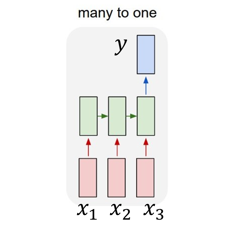
Firstly, let’s discuss how an input to the network looks like. A model takes a sequence of samples (observations) as an input and returns a single number (result) as an output. I call one sequence of observations a batch. Thus, a single batch is an input sequence to the network. Parameter timesteps defines the length of a sequence. This means that the number of timesteps is equal to the number of samples in a batch. Additionally, since our input has only one feature, the dimension of the input is set to one.
Mathematically, we may say that a batch \(x\) is a vector \(x\in \Bbb{R}^{timesteps}\) and the model outputs a value \(y\in \Bbb{R}\).
According to the classification done by Andrej Karpathy, we call such a model a many-to-one model . Let’s say that that our timesteps parameter equals 3. This means that an arbitary sequence of a length three \(x=\begin{bmatrix}x_{1}\\x_{2}\\x_{3}\end{bmatrix}\) returns a single value \(y\) as shown below:
Finally, we define usual neural network parameters such as the number of LSTM layers and amount of hidden units in every layer. Our parameters are set to:
- timesteps = 20
- no_of_batches = 150
- no_of_layers = 3
- no_of_units = 10
For simplification we assume that every LSTM layer has the same number of hidden units. Many-to-one model requires, that after passing through all LSTM layers the intermediate result is finally processed by a single dense layer, which returns the final value \(y\). That implies that our neural network has the following architecture:
| Layer (type) | Output Shape | Param # |
|---|---|---|
| lstm_1 (LSTM) | (None, 20, 10) | 480 |
| lstm_2 (LSTM) | (None, 20, 10) | 840 |
| lstm_3 (LSTM) | (None, 10) | 840 |
| dense_1 (Dense) | (None, 1) | 11 |
By the way, we can directly see that the shape of the array which is being propagated during the foreward pass in LSTM layers depends on the parameters (no_of_units and timesteps).
Retrieving weight matrices from the Keras model
def import_weights(no_of_layers, hidden_units):
    layer_no = 0
    for index in range(1, no_of_layers+1):
        for matrix_type in ['W', 'U', 'b']:
            if matrix_type != 'b':
                weights_dictionary["LSTM{0}_i_{1}".format(index, matrix_type)] = model_weights[layer_no][:,:hidden_units]
                weights_dictionary["LSTM{0}_f_{1}".format(index, matrix_type)] = model_weights[layer_no][:,hidden_units:hidden_units * 2]
                weights_dictionary["LSTM{0}_c_{1}".format(index, matrix_type)] = model_weights[layer_no][:,hidden_units * 2:hidden_units * 3]
                weights_dictionary["LSTM{0}_o_{1}".format(index, matrix_type)] = model_weights[layer_no][:,hidden_units * 3:]
                layer_no = layer_no + 1
            else:
                weights_dictionary["LSTM{0}_i_{1}".format(index, matrix_type)] = model_weights[layer_no][:hidden_units]
                weights_dictionary["LSTM{0}_f_{1}".format(index, matrix_type)] = model_weights[layer_no][hidden_units:hidden_units * 2]
                weights_dictionary["LSTM{0}_c_{1}".format(index, matrix_type)] = model_weights[layer_no][hidden_units * 2:hidden_units * 3]
                weights_dictionary["LSTM{0}_o_{1}".format(index, matrix_type)] = model_weights[layer_no][hidden_units * 3:]
                layer_no = layer_no + 1

    weights_dictionary["W_dense"] = model_weights[layer_no]
    weights_dictionary["b_dense"] = model_weights[layer_no + 1]
Our next step involves extracting weights in form of numpy arrays from the Keras model. For every LSTM layer created in our Keras model, the method returns three arrays:
- first array (a kernel) stores weights which correspond to \(W\) weights for each of four LSTM gates: input gate, forget gate, cell state gate and output gate.
- second array (called a reccurent kernel) contains respective \(U\) weights
- the last, third array (bias) stores respective \(b\) values.
Function import_weights allows us to quickly extract weights from the Keras model and store them in weights_dictionary, where keys of the dictionary are array names and values are the respective numpy arrays. Taking into account the nature of our model, the last component of the network is a dense layer, so we additionally read off weights for that element.
Defining a model in Keras
class LSTM_Keras(object):
    def __init__(self, no_hidden_units, timesteps):
        self.timesteps = timesteps
        self.no_hidden_units = no_hidden_units
        model = Sequential()
        model.add(LSTM(units = self.no_hidden_units, return_sequences = True, input_shape = (self.timesteps, 1)))
        model.add(LSTM(units = self.no_hidden_units, return_sequences = True))
        model.add(LSTM(units = self.no_hidden_units, return_sequences = False))
        model.add(Dense(units = 1))
        self.model = model
The object of the class LSTM_Keras returns a model of a neural network. We need this element to:
- obtain weights for our custom-made model.
- compare results between Keras implementation and our custom-made implementation.
Defining our custom-made model
class custom_LSTM(object):

    def __init__(self, timesteps, no_of_units):
        self.timesteps = timesteps
        self.no_hidden_units = no_of_units
        self.hidden = np.zeros((self.timesteps, self.no_hidden_units),dtype = np.float32)
        self.cell_state = np.zeros((self.timesteps, self.no_hidden_units),dtype = np.float32)
        self.output_array = []

    def hard_sigmoid(self, x):
        slope = 0.2
        shift = 0.5
        x = (x * slope) + shift
        x = np.clip(x, 0, 1)
        return x

    def tanh(self, x):
        return np.tanh(x)

    def layer(self, xt, Wf, Wi, Wo, Wc, Uf, Ui, Uo, Uc, bf, bi, bo, bc):
        ft = self.hard_sigmoid(np.dot(xt, Wf) + np.dot(self.hidden, Uf) + bf)
        it = self.hard_sigmoid(np.dot(xt, Wi) + np.dot(self.hidden, Ui) + bi)
        ot = self.hard_sigmoid(np.dot(xt, Wo) + np.dot(self.hidden, Uo) + bo)
        ct = (ft * self.cell_state)+(it * self.tanh(np.dot(xt, Wc) + np.dot(self.hidden, Uc) + bc))
        ht = ot * self.tanh(ct)
        self.hidden = ht
        self.cell_state = ct
        return self.hidden

    def reset_state(self):
        self.hidden = np.zeros((self.timesteps, self.no_hidden_units),dtype = np.float32)
        self.cell_state = np.zeros((self.timesteps, self.no_hidden_units),dtype = np.float32)

    def dense(self, x, weights, bias):
        result = np.dot(x, weights)+bias
        self.result=result[0]
        return result[0]

    def output_array_append(self):
        self.output_array.append(self.result[0])
The class custom_LSTM is the core of the code. Its task is to simulate a single LSTM layer in our network. The method layer is the actual implementation of the LSTM equations:
\[f_t=\sigma(W_f*x_t+U_f*h_{t-1}+b_f)\] \[i_t=\sigma(W_i*x_t+U_i*h_{t-1}+b_i)\] \[o_t=\sigma(W_o*x_t+U_o*h_{t-1}+b_o)\] \[c_t={f_t}\circ{c_{t-1}}+i_t*tanh(W_c*x+U_c*h_{t-1}+b_c)\] \[{h_t=o_t * tanh(c_t)}\]The basic functionality of the custom-made LSTM layer is
- change the internal state during forward propagation of the batch
- return an intermediate (hidden) result, which flows from LSTM cell (layer) to the consecutive layer.
The thing which surprised me while I was reading the Keras source code, is that an ordinary sigmoid function has been replaced by a hard sigmoid. The standard logistic function may be sometimes slow to compute because it requires calculating the exponential function. Usually the high-precision result is not needed and an approximation suffices. This is why the hard sigmoid is being used here, to approximate the standard sigmoid and accelerate the computation.
Additional methods of the class allow us to:
- reset state of a layer.
- implement the dense layer, which returns a final output.
Implementation
for batch in range(input_to_keras.shape[0]):

    LSTM_layer_1.reset_state()
    LSTM_layer_2.reset_state()
    LSTM_layer_3.reset_state()

    for timestep in range(input_to_keras.shape[1]):

        output_from_LSTM_1 = LSTM_layer_1.layer(input_to_keras[batch,timestep,:], weights_dictionary['LSTM1_f_W'], weights_dictionary['LSTM1_i_W'],
                                                                                  weights_dictionary['LSTM1_o_W'], weights_dictionary['LSTM1_c_W'],
                                                                                  weights_dictionary['LSTM1_f_U'], weights_dictionary['LSTM1_i_U'],
                                                                                  weights_dictionary['LSTM1_o_U'], weights_dictionary['LSTM1_c_U'],
                                                                                  weights_dictionary['LSTM1_f_b'], weights_dictionary['LSTM1_i_b'],
                                                                                  weights_dictionary['LSTM1_o_b'], weights_dictionary['LSTM1_c_b'])

        output_from_LSTM_2 = LSTM_layer_2.layer(output_from_LSTM_1, weights_dictionary['LSTM2_f_W'], weights_dictionary['LSTM2_i_W'],
                                                                    weights_dictionary['LSTM2_o_W'], weights_dictionary['LSTM2_c_W'],
                                                                    weights_dictionary['LSTM2_f_U'], weights_dictionary['LSTM2_i_U'],
                                                                    weights_dictionary['LSTM2_o_U'], weights_dictionary['LSTM2_c_U'],
                                                                    weights_dictionary['LSTM2_f_b'], weights_dictionary['LSTM2_i_b'],
                                                                    weights_dictionary['LSTM2_o_b'], weights_dictionary['LSTM2_c_b'])

        output_from_LSTM_3 = LSTM_layer_3.layer(output_from_LSTM_2, weights_dictionary['LSTM3_f_W'], weights_dictionary['LSTM3_i_W'],
                                                                    weights_dictionary['LSTM3_o_W'], weights_dictionary['LSTM3_c_W'],
                                                                    weights_dictionary['LSTM3_f_U'], weights_dictionary['LSTM3_i_U'],
                                                                    weights_dictionary['LSTM3_o_U'], weights_dictionary['LSTM3_c_U'],
                                                                    weights_dictionary['LSTM3_f_b'], weights_dictionary['LSTM3_i_b'],
                                                                    weights_dictionary['LSTM3_o_b'], weights_dictionary['LSTM3_c_b'])

    LSTM_layer_3.dense(output_from_LSTM_3, weights_dictionary['W_dense'], weights_dictionary['b_dense'])
    LSTM_layer_3.output_array_append()
Having defined all the helper functions and classes, we can finally implement our custom-made LSTM (main part of the code).
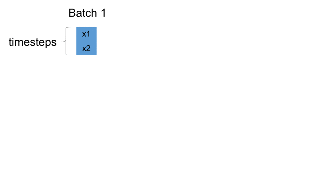
Firstly, we initialize a model in Keras. The weights are automatically created using default settings (kernel weights initialized according to Xavier’s initialization, recurrent kernel weights initialized as a random orthogonal matrix, bias set to zero). Secondly, we create three custom-made LSTM layers. Thirdly, we create an input to the network. It is a sequence of a pre-defined size of random integers in range 0 to 100. Finally, we start a loop, which computes the result of our custom-made neural network. To illustrate the flow of variables for a sample network, which takes batches of two samples, please see figure below:
For every batch, when all samples have passed through the architecture, the last sample enters the dense layer. This results in the final output for the given batch. Additionally, the state of every LSTM layer is reset. This is to simulate what happens in Keras after each batch has been processed. By default, when defining an LSTM layer, the argument stateful= False. If it were True,
the last state for each sample a batch would be used as initial state for the first in the following batch.
In our case, for every new batch the internal state of every LSTM cell is being reset. Now every output \(y\) returned by a given batch is being appended to the list output_array. This structure holds results returned by our network for every batch of observations. Having all results saved to one list, we may now compare our solution with the one returned by Keras.
Comparison and summary
We run the code with the specified parameters. One can immediately observe, that by playing with the parameters (increasing the number of timesteps, batches and layers), we radically increase the runtime. In practice it is much more efficient to do the prediction (forward propagation) step directly in Keras. In the end, smart implementation aces our sluggish for-loops out. Our complicated and time-consuming implementation may be wrapped up by a single line of code in Keras:
model.predict (x)
Let’s take a look at the results:

result_custom = [-0.0865001, -0.0895177, -0.0988678, … ]
result_keras = [-0.0865001, -0.0895177, -0.0988678, …]
We see that our implementation and results returned by Keras match very accurately (up to eight decimal places)! This is only a basic breakdown of an basic LSTM model. It has simple, numerical data with a single feature as an input. Still, the code should give a good insight (a glimpse under the hood) into the mathematical operations behind LSTMs.
The full code in Python
For condensed, full code please visit my github.