
Understanding AlphaGo Zero [1/3]: Upper Confidence Bound, Monte Carlo Search Trees and Upper Confidence Bound for Search Trees
Being interested in current trends in Reinforcement Learning I have spent my spare time getting familiar with the most important publications in this field. While doing the research I have stumbled upon the AlphaGo Zero course by Depth First Learning group. I love how they structure their courses as self-contained lesson plans focusing on deep understanding of the theory and provide background behind every approach. So far they offer just three courses, but their quality is outstanding. It is also great that they provide related reading for further study. I have decided to follow their AlphaGo Zero course and publish my learnings in form of three blog posts. Every entry will be tightly correlated with the topics from the curriculum. Note that the articles will not follow the order suggested by the authors of the course.
This first entry will discuss the concepts of Upper Confidence Bound (UCB), Monte Carlo Search Trees (MCST) and Upper Confidence Bound for Search Trees (UCT). I will not only examine the theory behind concept but also implement them in Python. In the end my final goal is not only to understand the method but also be able to use it in practice.
I assume that the reader has some prior knowledge pertaining the fundamentals of reinforcement learning.
Upper Confidence Bound
One of the simplest policies for making decisions based on action values estimates is greedy action selection.
\[A_t = \underset{a}{\mathrm{argmax}}(Q_t(a))\]This means, that in order to choose an action \(A_t\) we compute an estimated value of all the possible actions and pick the one which has the highest estimate. This greedy behavior completely ignores the possibilities that some actions may be inferior in the short run but ultimately superior in the longer perspective. We can fix this shortcoming by deciding that sometimes (the “sometimes” is parametrized by some probability \(\epsilon\)) we simply ignore the greedy policy and pick a random action. This is the simplest way to enforce some kind of exploration in this exploitation-oriented algorithm. Such a policy is known as epsilon-greedy.
Even though epsilon-greedy policy does help us to explore the non-greedy actions, it does not model the uncertainty related to each action. It would be much more clever to make decisions by also taking into account our belief, that some action value estimates are much more reliable i.e. they are closer to some actual, unknown action value \(q_{*}(a)\) then others. Even though we do not know \(q_{*}(a)\) (it is actually our goal to estimate it), we can use the notion of the difference between the desired \(q_{*}(a)\) and currently available \(Q_t(a)\). This relationship is described by the Hoeffding’s Inequality.
Imagine we have \(t\) independent, identically distributed random variables, bounded between 0 and 1. We may expect that their average is somewhat close to the expected value. The Hoeffding’s inequality precisely quantifies the relationship between \(\bar{X_t}\) and \(\mathbb{E}[X]\).
\[Pr[|\bar{X_t}-\mathbb{E}[X]|>m] \leq e^{-2tm^2}\]The equation states that the probability that the sample mean will differ from its expected value by more then some threshold \(m\) decreases exponentially with increasing sample size \(t\) and increasing threshold \(m\). In other words, if we want to increase the probability that our estimate improves, we should either collect more samples or agree to tolerate higher possible deviation.
In our multi-armed bandit problem we want to make sure that our estimated action value is not far from the real action value. We can express the threshold \(m\) as a function of an action and call it \(U_t(a)\). This value is known as an upper confidence bound. Now, we can apply the Hoeffding’s inequality and state:
\[Pr[|Q_t(a)-q_*(a)|> U_t(a)] \leq e^{-2tU_t(a)^2}\]Let’s denote this probability as some very small number \(l\) and transform this expression.
\[l = e^{-2N_tU_t(a)^2}\] \[U_t(a) = \sqrt{-\log{l}/2N_t(a)}\]We can make \(l\) dependent on the number of iterations (let’s say \(l = t^{-4}\)) and rewrite the equation.
\[U_t(a) = \sqrt{-\log{t^{-4}}/2N_t(a)} = C\sqrt{\log{t}/{N_t(a)}}\]Finally, we can write down the UCB policy:
\[UCB(a) = \underset{a}{\mathrm{argmax}}(Q_t(a) + C\sqrt{\log{t}/{N_t(a)}})\]The choice of \(l\) is in practice reflected by the parameter \(C\) in front of the square root. It quantifies the degree of exploration. With the large \(C\) we obtain greater numerator value of the square root and make the uncertainty expression more significant with respect to the overall score \(UCB(a)\). However, ultimately \(U_t(a)\) is bound to decay, since the numerator (\(N_t(a)\) - number of times we have chosen action \(a\)) increases with the higher rate then the numerator.
We may write down a pseudo-code for a simple, multi-armed bandit algorithm (UCB1) :
Initialize a Bandit with:

p # arm pull number
a # possible actions a
c # degree of exploration

Q(a) = 0	# action value estimates
N(a) = 0	# number of times the actions are selected
t = 0

for pull in range(p):
	t = t + 1
	# choose an action according to UCB formulation
	A = argmax(Q(a) + c*sqrt(ln(t)/N(a)))

	R = Bandit(A)			# receive a reward from the environment
	N(A) = N(A) + 1			# update the action selection count
	Q(A) = Q(A) + (R-Q(A)/N(A)	# update action value estimate
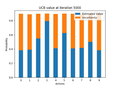
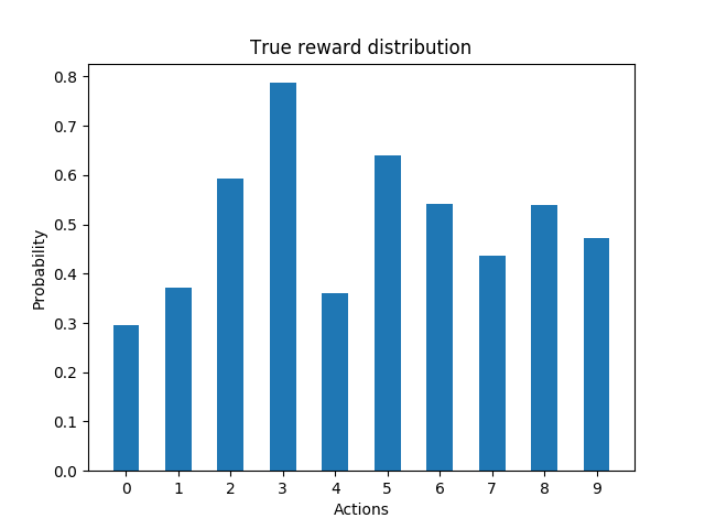
Finally, I have implemented UCB1 algorithm in Python: you can find the code here. I have tested it for a bandit with ten arms and 100 runs. Note, that that my implementation makes algorithm do some random exploration, it is not pure vanilla UCB1.
The following diagrams illustrate how the algorithm incrementally estimates the probability of receiving a reward from each of the arms for one single run.
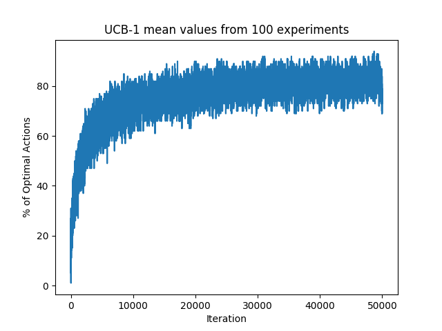
Next experiment involves running the algorithm 100 times and computing the percentage of optimal actions taken for each iteration of UCB1.
MCST & UCT
Monte Carlo Search Tree (MCST) is a heuristic search algorithm for choosing optimal choices in decision processes (this includes games). Hence, theoretically it can be applied to any domain that can be described as a (state, action) tuple.
In principle, the MCST algorithm consists of four steps:
-
Selection: the algorithm starts at the root node R (initial state of the game) and traverses the decision tree (so it revisits the previously “seen” states ) according to the current policy until it reaches a leaf node L. If node L:
a) is a terminal node (final state of the game) - jump to to step 4.
b) is not terminal, then it is bound to have some previously unexplored children - continue with step 2.
-
Expansion: We expand one of the child nodes of L - let’s call this child node C.
-
Rollout: Starting from node C, we let the algorithm simply continue playing on it’s own according to some policy (e.g random policy) until we reach a terminal node.
-
Update: Once we reach a terminal node, the game score is returned. We propagate it (add it to the current node value) through all the nodes visited in this iteration (starting with C, through all the nodes involved in selection step, up to the root node R). We do not only update the node value, but also the number of times each of the nodes has been visited.
Wait a minute… Since each node keeps the information about its value and number of times it has been visited, we may use UCB to choose the optimal action for every node. The UCT (Upper Confidence Bound for Search Trees) combines the concept of MCST and UCB. This means introducing a small change to the rudimentary tree search: in selection phase, for every parent node the algorithm evaluates its child nodes using UCB formulation:
\[UCT (j) =\bar{X}_j + C\sqrt{\log(n_p)/(n_j)}\]Where \(\bar{X}_j\) is an average value of the node (total score divided by the number of times the node has been visited), \(C_p\) is some positive constant (responsible for exploration-exploitation trade-off), \(n_p\) is the number of times the parent node has been visited and \(n_j\) is the number of times the node \(j\) has been visited.
The algorithm has useful properties. It not only requires very little prior knowledge about the game (apart from the legal moves and game score for terminal states) but effectively focuses the search towards the most valuable branches. We may also tune it in order to find a good trade-off between the algorithm speed and number of iterations. This is quite important since MCST gets pretty slow for large combinatorial spaces.
If you would like to implement UCT from the scratch I can highly recommend the code presented in MCST research hub (link below). The authors have provided code snippets in Python and Java together with a template to create your own small games that can be “cracked” using UCT.
I have modified the code and created an A.I opponent for 4x4 tic tac toe. Every time the adversary is prompted to make a move, it runs 1000 UCT iterations in order to find the best action. I must admit that the opponent is quite difficult to beat. During the game play I am being successfully blocked by the A.I. UCT allows it to quickly come up with simple, effective strategies.
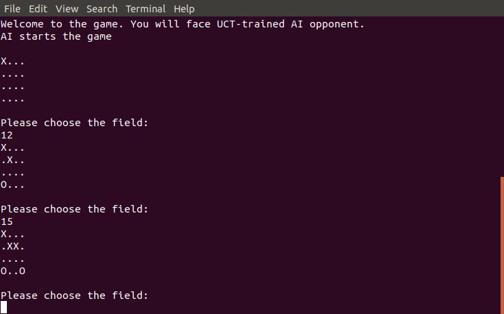
The source code can be found in the github repo.
Sources:
UCB
Sutton & Barto book: Sections 2.1 - 2.7 - excellent introduction to multi-armed bandit approaches.
Blog post by Lilian Weng - short and concise introduction to basic algorithms used in multi-armed bandit.
Blog post by Jeremy Kun - a bit more detailed (but super interesting) analysis of UCB.
MCST
MCTS research hub - excellent starting point for getting familiar with the algorithm.
UCT video tutorial by John Levine - short and clear explanation of MCST, together with a worked example.