
Option Pricing - Introduction, Example and Implementation
Option Pricing: Introduction, History and Implementation
This blog post is more focused on the financial, rather than software, engineering. It touches upon one of the most common financial derivatives - options. In the write-up I will briefly introduce two basic options (calls and puts), show one of their fundamental applications in financial engineering, and finally discuss my implementation of two option pricing models - Black-Scholes formula and Binomial Option Pricing Model. For the analysis, I use two assets, Tesla and Coca-Cola stocks.
Introduction
So you are a stock trader, who believes that the price of some stock, let’s say Tesla, will rise over next four weeks. Why would you suppose that? Maybe you are expecting that due to the new, impressive OS update, their vehicles may become far superior to competition’s product. This should bump the number of Teslas sold and drive TSLA’s stock price up, ultimately making you pocket a handsome profit.
But you are a smart investor, aware of the possible trouble ahead. You know that Tesla is in the volatile automotive business. On one hand you are interested in the company. On the other hand, you are aware of the industry risk, since it may be directly influence the performance of your stock.
Options can be used as as an “insurance” to your position. This strategy is also known as hedging. Hedging is employed to minimise any losses resulting from an investment position. One of the simplest hedging methods is to use a put option. A put option is a contract that allows you to sell a stock at a pre-determined price (a.k.a a strike price), on or before a given date. By employing “protective put” (or “married put”), an investor can basically defend himself against theoretical stock plunge. There is no free lunch though, “buying” the insurance means, that we sacrificing some of the possible excess gains.
Practical Example
As of today, one share of TSLA is $545. At the same time, you purchase a put to insure the purchased stock. The strike price of the option should be at least greater than the amount you paid for the actual stock. For example, you buy put with a strike price of $550, with additional premium of $60 per share, which expires in four weeks.
We can plot the risk characteristics of such a strategy.
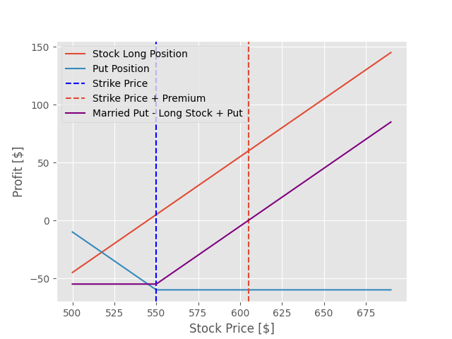
We can see that for a stock, the theoretical profit (and loss) are not bounded. Worst case scenario, you can simply loose all your money. Best case scenario, you may enjoy unlimited wealth increase. For a put, its is agreed upon that once the stock price falls below the strike price, you enjoy a linear profit (i.e you bet on stock price plummeting). If the stock price rises above the strike price, you may choose not to excercise the option and loose nothing. Of course, this kind of free, wonderful insurance is too good to be true in reality. That is why investors pay substantial premiums for the insurance - in this particular case, the premium amounts to mind-boggling 11%. As a result, the curve is shifted downwards by the premium price.
Now, by combining long position and put, we simply add two curves and observe the effect of the marriage between the long position and the put:
- If the stock price is higher then the initial stock price (when you bought the equity) + premium, you start enjoying linear profit from your investment, congratulations!
- If the stock price is lower then the initial stock price + premium, you will experience losses proportional to the fall in stock price.
- However, the moment the stock price falls below the strike price, the lower bound on our losses kicks in. From this moment on, you will not loose any more money. This is the put protecting you from any possible troubles.
Note, that married put has similar effect as the call option. It basically hedges your long position. In fact, an investor can mix long positions, short positions and various options to create different strategies to hedge against different risks. The ingenuity of financial engineers gave rise to constructs with such names as butterfly spread, iron condor or straddle, but those are advanced products not covered in this write-up.
The (un)Solved Mystery of Option Pricing
Option pricing turns out to be much more interesting then figuring out the value of bonds or stocks. Calculating the current value of the option, has baffled the financial world for a long time. The history of solving the problem stretches throughout the whole twentieth century and, quite frankly, could make a great Netflix series plot.
It starts with a doctoral thesis by a French PhD student, Louis Bachelier. The pioneer of mathematical finance was writing his dissertation on options on Paris stock exchange. One of his biggest achievements is the development of the random walk hypothesis - financial theory stating that the stock market prices evolve according to a random process modeled by the Brownian motion. His discoveries had very interesting ramifications.
First of all, it was a rare example of the situation, where an economist comes up with an idea, which only later is adopted by a physicist. And not just any physicist, but Albert Einstein himself. His work, which also used the concept of Brownian motion, has been awarded with the Nobel Prize.
There was another beautiful coupling between physics and economy hidden in Bachelier’s work. The student has shown that the same family of PDEs which dictate how the heat distribution evolves over time in a solid medium, can tell us how the value of an option changes with respect to the value of the underlying asset and time. It is stunning that a purely physical theory developed by Fourier, does describe the financial markets so accurately!
Just to demonstrate - the heat equation for the 1D body (e.g. metal rod):
\[\frac{\partial u}{\partial t} = \alpha \left( \frac{\partial^2 u}{\partial x^2}\right)\]…versus the final Black-Scholes equation:
\[\frac{\partial V}{\partial t}= -\frac{1}{2}\sigma^2 S^2 (\frac{\partial^2 V}{\partial S^2}) - rS\frac{\partial V}{\partial S} + rV\]Finally, it took almost 100 years for the brightest minds (among them PhDs from Yale and MIT) of the mathematics to actually solve the option pricing model. The duo Black and Scholes, but also an economist Robert Merton, came up independently with the solution, for which they have been awarded by a joint Noble prize. While the gentlemen received accolades for their research endeavours, Edward Thorp has managed to use Bachelier’s framework several decades earlier. He has done it while managing an extremely successful hedge fund at Princeton Newport Partners. Finally, not only Thorp, but probably many financial engineers has benefited from arbitrage opportunities unlocked by the option pricing formula.
My Implementation of Option Pricing Mechanisms
Black-Scholes Formula
It is a truly fascinating process to go through the derivation of the Black-Scholes formula. Starting from the definition of the Brownian motion, one uses Taylor’s expansion to acquire the Black-Scholes differential equation and finally, by employing fundamentals of PDEs (including initial and boundary condiitons, particular structure of equation), one shall reach the final result:
\[V(S, t)= N( d_1) S - N(d_2)K e^{-rt}\]where:
\[d_1= \frac{1}{\sigma \sqrt{ t}} \left[\ln{\left(\frac{S}{K}\right)} + t\left(r + \frac{\sigma^2}{2} \right) \right]\] \[d_2= \frac{1}{\sigma \sqrt{ t}} \left[\ln{\left(\frac{S}{K}\right)} + t\left(r - \frac{\sigma^2}{2} \right) \right]\]From the model we are able to calculate the price of an option based on a number of different factors. To use Black-Scholes formula, we need first to figure out the value of the parameters of the equation:
- \(K\), the strike price. If we decide to buy an option, this what we obviously should now. This is our bet on the future price of the asset.
- \(T\), time to maturity is also known. This is when the option expires.
- \(\sigma\), the volatility. There are two ways to compute this value. We may retrieve the implied volatility from the current available options on the market for the same asset. Alternatively, and this is the approach in my implementation, we may use historical volatility- the standard deviation of log returns (difference of closing prices of the stock over consecutive days) over past data. The volatility is annualized to be consistent with the rest of the data.
- \(r\), annualized risk-free rate. In my implementation, this is the mean of the current interest rates on US treasury bill rates for different times of maturity.
Finally, \(N(.)\) is cumulative distribution function.
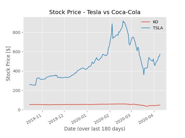
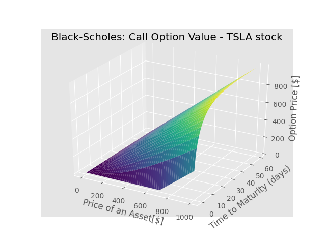
Let’s scrutinize two stocks with very different characteristics - volatile, young Tesla and steady, blue chip - Coca-Cola. As shown on the diagram above, there is little dispersion in the price of Coca-Cola. Tesla, on the contrary, is one of the hottest and most volatile stocks of the recent years. Please note that my results may be very particular. Due to the current situation on the markets, most of the stocks are characterised by unusually high volatility. At the same time, we are naturally experiencing very low interest rates. The options chosen are calls. The price of the premium is neglected, as well as the fact that KO pays regular dividends.
INFO:root:
 Today on 2020-04-09 00:00:00,
 TSLA stock price is 573.0.
 We agree on strike price 687.6.
 Interest rate is: 0.242%, 180 days historical volatility is 0.83
 The call matures in 60 days.
INFO:root:
 Today on 2020-04-09 00:00:00,
 KO stock price is 49.0.
 We agree on strike price 58.8.
 Interest rate is: 0.242%, 180 days historical volatility is 0.34
 The call matures in 60 days.
Both plots tell us, how the function \(V(S,t)\) behaves for a given pair of variables. One can observe that, for fixed \(t\), the price of the option increases as the stock price increases. This makes sense, since it is increasingly more likely to expire with a positive value. Also, for fixed \(S\) and decreasing \(t\) (meaning we are approaching maturity), the call becomes worth less and less, since its value at expiration is become more and more certain. This means that the more volatility an option has, the more expensive it is. Why? Uncertainties are costly. Since costs raise prices, and volatility is an uncertainty, volatility raises prices.
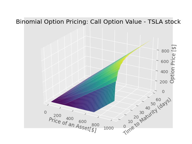
Binomial Option Pricing Model
For some applications, option pricing can be performed using the Binomial Option Pricing Model (BOPM). Both BOPM and Black-Scholes approach are built on the same assumptions. As a result, the binomial model provides a discrete time approximation for the continuous process underlying the Black–Scholes model. The binomial model assumes that movements in the price follow a binomial distribution. The derivation of BOPM is much more straightforward then the mathematics behind Black-Scholes. The final formula here is:
\[V(S,t)=r^{-t}\sum_{k=0}^{t}\binom{t}{k}p^k(1-p)^{t-k}\max{(0, u^k d^{t-k}S-K)}\]where:
\[p = \frac{r-d}{u-d}\]And \(u\) and \(d\) are specific factors of the asset price moving move up or down. Those can be deduced from the implied or historical volatility.

As shown below, BOPM provides a good, discrete approximation to the Black-Scholes model.
Additional Reading
- The Man Who Solved the Market: How Jim Simons Launched the Quant Revolution, Gregory Zuckerman
- A Non-Random Walk Down Wall Street, Andrew Lo
- Options, Futures, and Other Derivatives, John C. Hull