
Mixed Martial Maths - Simple Reasoning Tools For Complex Phenomena
Recently I have been interested in obtaining a very particular skill. I have seen this ability demonstrated by many excellent individuals - not in only in the tech world, but also in finance or consulting industry. I am talking here about the art of back-of-the-napkin (or back-of-the-envelope) calculation, also known as guesstimation or order-of-magnitude analysis.
In your professional and private life you may be often presented with difficult question, where the insight is much more important than the precision of the final answer. For example:
How many weddings are performed each day in Japan?
or
How many total miles do Americans drive in a year?
The challenge lies in the complexity of the problem, not in the quality of the obtained result. Giving the exact answer to any of those riddles is the least important thing. The crucial issue is: how to even begin answering the question?
Those challenges, at least in the context of engineering or physics, are called Fermi problems. Surprisingly, there are many professions where one may grapple with those type of questions on the daily basis:
- consultants, who are often asked to estimate the size of something with no, or little, data available.
- software engineers, who need to approximate the task complexity to efficiently plan new development of features and release timelines.
- economists, who often use incomplete information to create economic forecasts.
- scientists, who look for estimates for the problem before turning to more sophisticated methods calculate a precise answer.
- engineers, who use low-cost thought experiments to test ideas before committing to them.
Science and engineering, our modern ways of understanding and altering the world, are said to be about accuracy and precision. But accuracy and precision are what modern computers are for. Humans are indispensable when it comes to insight.
Even though we improve our insight through experience and knowledge, the complexity is what makes our “mental registers overflow” and wash away all the understanding. The goal of this article is to present several reasoning tools, which will allow you to harness the complexity of the modern world and make you less wrong on the daily basis.
Motivation and Further Reading
Over the past year I was actively trying to improve my general problem solving ability, as well as train my brain to reason from first principles. I went through some impressive blog posts (you can never go wrong with waitbutwhy), YouTube videos (you can never go wrong with Grant Sanderson) and many helpful reddit threads. One of them mentioned Sanjoy Mahajan, an excellent MIT professor, who has been educating his students on the art of approximation for more than a decade. I have thoroughly studied his fascinating book: “The Art of Insight in Science and Engineering: Mastering Complexity”. Only recently I have discovered that his lectures are also available online. Long story short, I found the material fascinating and created a substantial amounts of messy study notes. I have decided to structure them in the form of list - a list of nine simple reasoning tools for harnessing complexity. I hope that the toolbox will also be useful for you my dear reader.
Tool # 1 Divide and Conquer
Let’s get familiar with the first reasoning tool. Whenever you are required to estimate some complex value, do not let the task formulation overwhelm you. Break hard problems into manageable pieces - divide and conquer!
Counting to a Billion
I will be mentioning divide-and-conquer reasoning in conjunction with other reasoning tools throughout this blog post. This is why I am just briefly introducing a simple problem to illustrate the point. Let’s answer the following question:
How long would it take to count to a billion?
The purpose of divide-and-conquer is to be break the problem into smaller, digestible pieces and then combine them into a full solution.
First let’s think about how long it takes to say a number out-loud. For relatively small numbers it takes me about 0.5 second, while I need up to 5 seconds to say: 999,999,999. We can use the best- and worse-case scenario to compute an “average” time necessary to say a number.
To combine quantities produced by our “mental hardware” (especially lower and upper bounds), we shall use geometric mean, rather than arithmetic mean. This is because geometric mean operates on a logarithmic scale and this is compatible with how humans perceive quantities - through ratios.
\[t_{mean} = \sqrt{t_{max} \cdot t_{min}}=\sqrt{5 \cdot 0.5} \approx 1.6s\]An average time to say a number out-loud is about 1.6 second. Now, we can complete the assignment by calculating how much time it takes to say a number out-loud billion times!
\[t_{tot} = t_{mean} \cdot 10^9 = 1.6s\cdot 10^9\]This is equivalent to about 51 years, quite some time!
We broke one, seemingly overwhelming problem into two, fairly easy ones. While the complexity of the example was pretty modest, the usefulness of divide-and-conquer reasoning will be demonstrated later on in this write-up.
Conclusion: No problem is too difficult! Use divide-and-conquer reasoning to dissolve difficult problems into smaller pieces.
Tool # 2 Harness the Complexity Using Abstractions
Divide-and-conquer reasoning is very useful, but not powerful enough on its own to deal with the complexity of the world.
And All That Jazz
Imagine that you just bought a huge collection of vinyl records. You are a very tidy person and want to organise your records in some orderly way. Surely, you do not want to spend hours looking for this one record every time you feel like playing something particular. Perhaps you could use divide-and-conquer to divide your newly acquired collection into groups, e.g. segregate the records by release date. However, it could be much more convenient to build some kind of structure or hierarchy for our collection. In our example, this could be grouping the records into genres. As the next step, we could expand this hierarchy and build tree-like representation of our collection by grouping jazz records into sub-genres: bebop, acid jazz, jazz rap.
Creating an adequate representation (abstraction) of the vinyl collection allows us to browse the complex structure quick and seamlessly.
When in Rome, Do Not Do As the Romans.
Have you ever noticed how ridiculously impractical, in the context of modern mathematics, Roman numerals are? It seems pointless to use them for any kind of useful algebra. XXVII times XXXVI is equivalent to \(27 \cdot 36\). However, because of the level of abstraction inadequate for this operation, it feels so unnatural to perform multiplication in this notation. The modern number system, based on the abstractions of value and zero, makes the operation surprisingly simple. Even if you cannot do mental multiplication fast, you could use its properties to compute:
\[27 \cdot 36 = (20+7) \cdot (30+6) = 20\cdot 30 + 7\cdot 30 + 20\cdot 6 + 7\cdot6 =\] \[=600+210+120+42=810+162=972\]But why did the Romans do, seemingly, such a poor job? You can find the answer here. The Romans were not concerned with pure mathematics, which usually requires high degree of abstraction. Instead they used mathematics to figure personal and government accounts, keep military records, and aid in the construction of aqueducts and buildings.
Conclusion: Good abstractions amplify our intelligence and bad abstractions make us confused. An example of good abstraction: “Could you slide the chair toward the table?”. An example of bad abstraction: “Could you, without tipping it over, move the wooden board glued to four thick sticks toward the large white plastic circle?”.
Tool # 3 Find What Remains Unchanged
Divide-and-conquer and abstractions help us to combat complexity by introducing order and structure. The upcoming tools help us to find some useful properties of the problem. Once the property is found, we are allowed to discard some portion of the complexity without any repercussions.
It is particularly beneficial to discover an existence of some invariants in the problem. Invariants mean that there exists some form of conservation or symmetry in the system. Hence, some part of complexity is a mirror copy of the remaining complexity and can be safely discarded.
A Rat-Eaten Chessboard
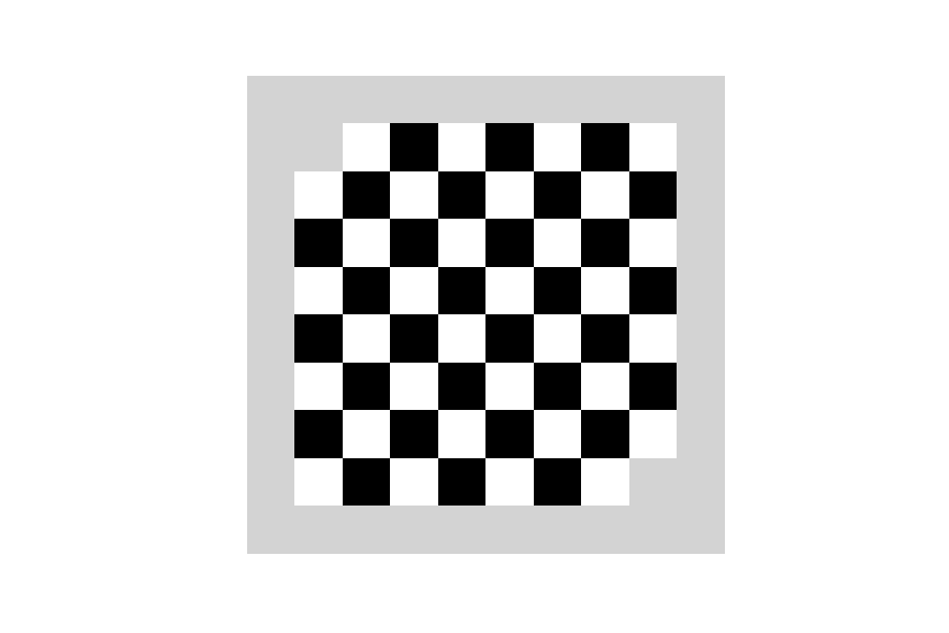
Imagine a basement, where you keep your old chess set. A rat comes out and gnaws on your antique chessboard. As a result, the animal chews off two diagonally opposite corners out your standard \(8 \times 8\) chessboard. In the basement you also keep a box of rectangular \(2 \times 1\) dominoes.
Can these dominoes tile the rat-eaten chessboard i.e. can we lay down the dominoes on the chessboard, so that every square is covered exactly once?
What we could try to do is to start placing dominoes naively, hoping that we spot some patterns or just stumble upon the solution. Most likely we would get overwhelmed by the number of possible move sequences. Instead of using brute force, let us identify some quantity, which remains unchanged, no matter how many dominoes pieces are on the board. In general, this quality is the invariant.
Since each domino covers exactly one white and one black square on the chessboard, the following relationship \(x\) between uncovered black squares and uncovered white squares remains unchanged. This is true, not matter how many dominoes are laying on the chessboard at any given time.
\[x = \text{uncovered}_{\text{white}} - \text{uncovered}_{\text{black}}\]A regular \(8 \times 8\) chessboard initially has 32 black squares and 32 white squares. Our perturbed chessboard is missing 2 black squares. This means that:
\[x_{initial} = 32-30=2\]Now, we succeed if there are no empty squares on the nibbled chessboard (and no overlapping dominoes). This means finishing the game with no uncovered white or black squares:
\[x_{final} = 0-0 = 0\]Because \(x_{final} \neq x_{initial}\) (\(x\) is always equal to 2 after every move until no further moves are available), we cannot tile the nibbled chessboard with dominoes. We can reach this conclusion immediately once we find a meaningful invariant.
Whenever facing a complex problem, it is helpful to look for the conserved quantity. Finding the invariant allows for creation of a high-level abstraction layer of the problem. Operating on this abstraction layer can directly lead to the solution without delving into the messy complexity of the problem at hand. Often, however, the invariant is given, so we can analyse the actions that preserve it. Those actions, which take advantage of the symmetry of the problem and preserve it, are called symmetry operations .
Carl Friedrich’s Math Assignment
The fans of mathematical anecdotes surely know the one about the young Carl Friedrich Gauss. As a young student he was given the following problem:
Find the sum numbers from 1 to 100.
It took just several minutes until the prodigy child quickly returned with the answer: 5050. What was the trick?
Gauss found the invariant, the sum, which does not change when the terms are added “forward” (from the lowest number to the highest) or “backward” (from the highest number to lowest) - hence he also discovered the corresponding symmetry operation.
\[S = 1+2+3+ \cdots + 99 + 98 + 100 = 100+99+98+\cdots+3+2+1\]Having found the symmetry of the problem, the solution is easy to compute. By adding the “forward” and backward” representation of the sum we end up with:
\[2S = 101+101+101+\cdots+101+101+101 = 101\cdot100\] \[S=\frac{10100}{2} = 5050\]Finding vertex without the calculus
Let’s find the maximum of the simple function:
\[f(x)=-x^2+2x\]Your instinct may tell you to use calculus to solve the problem, but why should we use a sledgehammer to crack a nut? Let’s do what Gauss did with a sum of series - use the invariant and related symmetry operation to crack the puzzle efficiently.
The invariant of the problem is the location of the minimum. We can safely guess that there is some symmetry available to be exploited (the equation represents a second-order polynomial, which has a parabolic shape).
We can factor the function:
\[f(x)=-x^2+2x=x(-x+2)\]Since multiplication is commutative (\(x(-x+2) = (-x+2)x\)) , we have found our symmetry operation: \(x \leftrightarrow -x+2\). This operation turns 2 into 0 or 3 into -1 (and vice-versa). The only value unchanged (left invariant) by the symmetry operation is 1, the solution to our problem!
Interestingly, I have also been recently reading completely unrelated book by Benoit Mandelbrot. It was interesting to stumble upon his testimony about invariants in the context of financial engineering:
Invariance makes life easier. If you can find some [market] properties that remain constant over time and place, you can build better and more useful models and maker sounder [financial] decisions - Benoit B. Mandelbrot, “The (mis)Behaviour of Markets”
Conclusion: When approaching a problem look for things which don’t change - the invariant or the conserved quantity. Finding it and taking advantage of the related symmetry often simplifies a complex problem.
Tool #4 Use Proportional Reasoning
Proportional reasoning is yet another powerful weapon, which allows to avoid complexity by taking a clever mental shortcut. Instead of spending time and effort to find some unknown quantity directly, we can estimate it through some relationship with the other, well-known quantity.
Counting McDonald’s Restaurants
If a person approached you on the street and asked: “how many McDonald’s restaurants are there in your country?”, you would be probably quite baffled. If not due to the surprising nature of the question, then certainly by the difficulty of the estimate. Most of the people I asked usually were overstating the number - some of the estimates were off by two orders of magnitude! They would surely give an accurate answer, if they knew about the proportional reasoning.
My hometown in Poland has, give or take, 400 thousand inhabitants. We surely had about 5 McDonald’s outlets back when I was attending middle high. Poland has population of 40,000,000. By applying simple proportional reasoning I can estimate that there are…
\[\text{restaurants}_\text{poland} = \text{restaurants}_\text{hometown}\cdot \frac{\text{population}_\text{poland}}{\text{population}_\text{hometown}} = 5 \cdot \frac{4 \cdot 10^7}{4 \cdot 10^5} = 500\]…McDonald’s restaurants in Poland. The actual number is 462 (data from 2019 according to wikipedia). Pretty neat huh?
To Fly or Not to Fly
Proportional reasoning can be effective, even when facing a seemingly daunting problem:
Which mean of transport is more fuel-efficient: a plane or a car?
A physicist or an economist could answer this question by applying full-fledged analysis, but there is no need to do so. The only required piece of domain knowledge is the high-school physics knowledge.
For cars travelling at highway speeds, most of the energy is consumed by fighting drag (air resistance). Planes on the other hand, not only need the energy to fight drag, but also to generate lift.
At a plane’s cruising speed, lift and drag are comparable. Lift plus drag is twice the lift alone. Neglecting lift ignores only a factor of two, which is fine for our approximation. As a result, we end up with two drag energies, one for a car and one for a plane.
To investigate, which mean of transport is more fuel-efficient, we can compute the ratio of drag energies for both vehicles. In general, drag energy of a body depends on its cross-sectional area, velocity and the density of the medium around that body:
\[\frac{E_{plane}}{E_{car}} = \frac{\rho_{plane}}{\rho_{car}} \cdot \frac{A_{cs, plane}}{A_{cs, car}} \cdot (\frac{v_{plane}}{v_{car}})^2\]Our goal is to find out the ratio on the left hand side. We can do this by estimating the terms on the right hand side.
Air density
Rather than estimating air density at the cruising altitude (plane) and at sea level (car) separately, let’s think about their ratio. Planes fly high - Mount Everest high. I know that climbers have difficulty breathing on the peak of the mountain due to lower oxygen density. This means that the density of the air decreases with altitude. Compared to the sea level, I am guessing the density ratio of 2 (sea level to plane’s cruising altitude).
Cross-section
Once again, we shouldn’t care much for each value separately. Let us directly estimate the ratio! How many car cross-sections can “fit” into a cross-section of a plane? I am pretty sure that in terms of width, plane’s round fuselage cross-section (I am neglecting the wings) could be occluded by three cars parked next to each other. Probably the same thing applies in the vertical dimension. If we stacked three cars on top of each other they could “cover” the plane horizontally. This means that the cross-section ratio is about \(3 \cdot 3 = 9\)

Velocities
Here, I feel pretty comfortable with estimating each velocity separately. A car travels at around 100km/h, while a plane travels at almost 1000km/h. This means velocity ratio of 10.
Finally, we can compute the drag energy ratio:
\[\frac{E_{plane}}{E_{car}} = \frac{1}{2} \cdot 9 \cdot (10)^2 = 450\]Given the common knowledge, that the fuel efficiency of a car and plane, per passenger, are roughly the same, I am pretty happy with this estimate. A car needs one “unit” of energy per person (assuming an average person drives to and from work alone). Conversely, a plane, which carries about 450 people, needs approximately one unit of energy per person as well.
Notice how divide-and-conquer, as well reasoning from first principles, were efficiently utilised in this analysis as well!
Conclusion: Instead of spending time and effort to compute some unknown quantity directly, try to estimate it (using proportions) through some other, related, well-known quantity.
Tool #5 Dimensional Analysis
Dimensional analysis makes it possible to say a great deal about the behaviour of a physical system - e.g. it facilitates the analysis of relationships between different physical quantities or even deduction of the underlying equations.
Dimensional Analysis “a la Huygens”
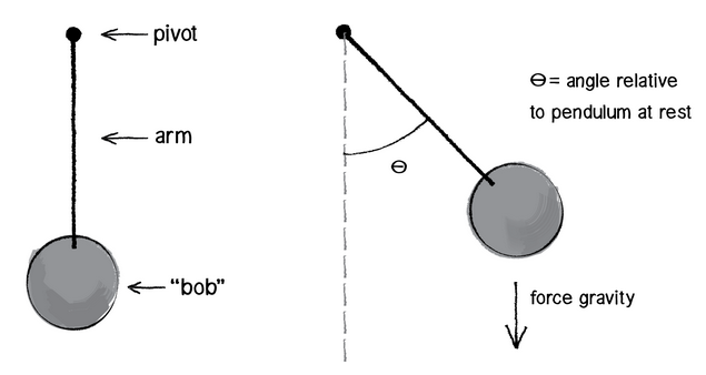
Let’s take a look at example which illustrates the basic method of dimensional analysis. Dimensional analysis, together with some physical intuition, allows us to find the equation for the period of oscillation for simple pendulum (a.k.a Huygens’s law for the period).
The procedure consists of 4 steps.
1. List relevant quantities
We make a list of all the physical variables and constants on which the answer might depend. Which quantities could influence the period of oscillation of the pendulum? Well, my intuition tells me that the mass of the bob matters, as well as the length of the string. The oscillation happens because the gravity is acting on the pendulum, so let’s account for that as well. To sum it up:
| Quantity | Symbol | Unit |
|---|---|---|
| period | \(T\) | \(s\) |
| gravity | \(g\) | \(\frac{m}{s^2}\) |
| mass | \(M\) | \(kg\) |
| length | \(L\) | \(m\) |
2. Form independent dimensionless groups
Those quantities shall be combined in the functional relation, such that the equation is dimensionally correct. How many independent relations (dimensionless group) are necessary to solve the problem? This is defined by the Buckingham Pi theorem:
Number of independent dimensional groups = number of quantities - number of independent dimensions
How many quantities do we have? Four - period, gravitational acceleration, mass and string’s length. How many independent dimensions do we have? Three - mass, time and distance. The acceleration is derived from distance and time so we do not consider it. We end up with 4-3=1 dimensional group.
Assume that the product of listed quantities, each raised to some unknown power, shall be dimensionless:
\[T^{\alpha}g^{\beta}M^{\gamma}L^{\theta} = C\]where \(C\) is some dimensionless constant.
3. Make the most general dimensionless statement
We solve system of four equations (choose the unknowns so that all the physical units in the equation cancel out) and obtain:
\[\alpha=2, \beta=1, \gamma=0, \theta=-1\] \[T^{2}g^{1}M^{0}L^{-1} = C \implies T = C\sqrt{\frac{g}{l}}\]We have found our dimensionless relation. Note that mass was actually superfluous and vanished in the process.
Also, note that the dimensionless constant \(C\) is universal. The same constant applies to a pendulum on Mars or a pendulum with a different string length. Once we find the constant, we can reuse it for the wide range of different applications.
4. Use physical knowledge to narrow down the possibilities
The last element is finding the dimensionless constant. How? Sure, you can solve the pendulum differential equation, but how about a small experiment? Take something which resembles a simple pendulum (e.g. I used my key chain) and make it oscillate. Write down the length and the period and plug it into equation to estimate \(C\). If the value is close to 6, well done! It is in fact \(2\pi\)!
A Picture Worth a Thousand Tons of TNT
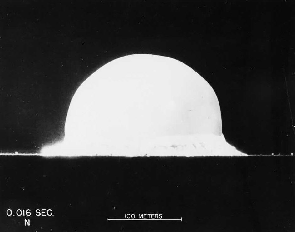
Estimating the period of the pendulum was just a warm up exercise. Time for something more exciting - estimation of the atomic bomb energy. Yes, this example will surely make us appreciate the power of the dimensional analysis.
The first explosion of an atomic bomb happened in New Mexico in 1945. Several years later a series of pictures of the explosion, along with a scale bar of the fireball and timestamps, were released out to the public. However, the information about the blast energy (yield) remained highly classified for years.
However, with the use of the pictures and the dimensional analysis, the great scientists G.I Taylor estimated the secret value pretty accurately.
Which quantities matter when it comes to the blast energy estimation? Let’s see what information does the photograph (above) provide us. Obviously the radius of the fireball at the given time point is valuable. The bigger the radius at the given time point, the greater the power of the explosion. What else matters? Probably the density of the surrounding medium, air.
| Quantity | Symbol | Unit |
|---|---|---|
| energy | \(E\) | \(\frac{kg \cdot m^2}{s^2}\) |
| time | \(t\) | \(s\) |
| radius | \(R\) | \(m\) |
| air density | \(\rho\) | \(\frac{kg}{m^3}\) |
Four quantities and three independent dimensions give us one independent dimensional group.
Once again, we solve a system of equations and compute the dimensionless relationship:
\[E^{\alpha}t^{\beta}R^{\gamma}\rho^{\theta} = C\] \[\alpha=1, \beta=2, \theta=-5, \gamma=-1\] \[E^{1}t^{2}R^{-5}\rho^{-1} = C \implies E = C\frac{\rho R^5}{t^2}\]Finding \(C\) in the analogous way to the previous example is difficult (unless you have some spare atomic bombs). I can spill the beans and tell you, that G.I Taylor estimated it (using experimental data) to be close to 1.
While air density can be looked up, the radius and time can be read off from the photograph. At t=0.016 seconds we can say that \(R \approx 150\) metres. Let’s plug in the numbers to find the energy.
\[E = \frac{1.2 \cdot 150^5}{0.016^2} \approx 10^{14}J\]\(10^{14}\) Joules is equivalent to 25 kilo-tons of TNT. Taylor has reported the value of 22 kilo-tons in 1950, while Fermi, who also used guesstimation to compute the yield obtained result of 10 kilo-tons in 1945. The actual, classified yield was 20 kilo-tons. Not bad for the back-of-the-envelope calculation…
Conclusion: Dimensional analysis allows us to establish the form of an equation, or more often, to check that the answer to a calculation as a guard against many simple errors.
Tool #6 Round and Simplify
The tools presented so far allowed for discarding complexity without any information loss. But when going gets tough, we need to sacrifice the quality (accuracy) of the obtained solution for the ability to quickly solve a task at hand.
Rounding to the Nearest Power of Ten
This application of approximation is incredibly simple, yet very effective. By rounding to the nearest power of ten, complex calculations boil down to addition and subtraction of integer exponents.
Let’s estimate the number of minutes in a month.
Let’s write down directly how many minutes are there in a 30 day month:
\[1\text{ month} \times \frac{30 \text{ days}}{\text{month}} \times \frac{24\text{ hours}}{\text{day}} \times \frac{60\text{ minutes}}{\text{hour}} = 30 \times 24 \times 60 \text{ minutes}\]You may find it quite challenging to multiply all the numbers quickly. So let’s round each factor to the nearest power of 10. For example, because 60 is a factor of almost 2 away from 100, but a factor of 6 away from 10, it gets rounded to 100. We apply same rule for the other factors:
\[30 \times 24 \times 60 \approx 10 \times 10\times 100 = 10^{1+1+2} = 10^4\]The exact value is 43,200, so the estimate of 10,000 is too small by 23 percent. This is a reasonable price to pay for the ability to estimate such a big number without any effort.
How High
By combining approximations and simplifications with previously mentioned tools - invariants and divide-and-conquer, we can easily find to answer to the following (tough) question:
How does the jump height of an animal depend on its size?
We want simple, so let’s not get involved into the unnecessary complexity. Start with the first simplification: assume that the animal starts from rest and directly jumps upward.
Fine, now we can try to start constructing some physical model to illustrate the problem. But which? The jump height seems to depend on so many factors: shape of the animal, amount of its muscles, efficiency of those muscles, whether the animal is bipedal or not and so on…
Once again, start simple. We may use principle of conservation to define two quantities:
-
\(E_\text{supplied}\) - the amount of energy needed for an animal to reach jumping height h.
-
\(E_\text{demanded}\) - the maximum amount of energy that an animal can generate using its muscles.
We can analyse both energy terms separately and then use the fact that they must be in equilibrium (like supply and demand in economics).

Energy demanded is the amount of energy needed for an animal to reach jumping height h. The type of energy, which is responsible for bodies being lifted up away from the Earth’s surface is potential energy. It depends on the height h, body mass \(m_\text{body}\) and gravity g. We can discard the gravity term - all the considered animals experience the same gravitational acceleration.
\[E_\text{demanded} \propto m_\text{body}h\]Energy supplied is the maximum amount of energy an animal can generate using its muscles. This energy is simply a product of the muscle mass \(m_\text{muscle}\) and the muscle energy density. Note that we are introducing another simplification: we treat all different muscles in the animal’s body as one, homogenous tissue: all the muscles contribute equally to the jump. We can go even further and say that the muscle energy density is the same for all the living creatures. Some might say that this is too much of a simplification, but my guts tells me otherwise: all muscles use similar “biological technology”. They have similar organic composition so why not treat them (approximately) equally? This assumption allows to consider the muscle energy density as constant so:
\[E_\text{supplied} \propto m_\text{muscle} \cdot \text{energy density}_\text{muscle} \propto m_\text{muscle}\]Neat. The next question is what is the relationship between the muscle mass \(m_\text{muscle}\) and body mass \(m_\text{body}\)? My guts tells me that this quantity does not only depend on the type of an animal (I would be surprised if this ratio was the same for a bull and a pig), but also on the age and gender (it would be different for an athletic male adult versus an old woman).
Once again, let’s simplify and throw away this information - treat the ratio as a constant. Yes, on hand we assume (courageously) that all animals have the same muscle to body mass ratio, but on the other hand we get to peel off the next layer of complexity.
\[E_\text{supplied} \propto m_\text{muscle} \propto m_\text{body}\]Now we can compare the demanded and supplied energy to obtain the following relationship:
\[m_\text{body}\propto m_\text{body}h\]Which means that jump height is in fact independent of the body mass of the animal!
\[m_\text{body}^0 \propto h\]How can this be true? Let’s think about it. Very small animals can jump very high. Think about insects such as fleas, grasshoppers or locust. But larger animals, such as crocodiles and turtles are very poor jumpers! Tigers, lions, humans and monkeys can jump very high. But can elephants jump at all? Let’s allow the data to provide some answers:
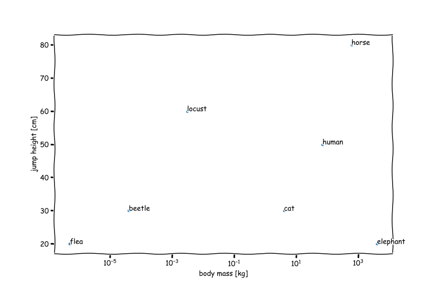
The data does in fact confirm our finding. For all the different animals, which mass spans from micrograms to tons (up to 8 orders of magnitude) the jumping height varies by tens of centimetres. The predicted scaling of constant \(m_\text{body}^0 \propto 1 \propto h\) is surprisingly accurate.
Conclusion: When the problem overwhelms you, do not be afraid to lower your standards. Approximate first, worry later. Otherwise you never start, and you can never learn that the approximations would have been accurate enough—if only you had gathered the courage to make them.
Tool #7 Consider Easy Cases First
A correct analysis works in all cases—including the simplest ones. This principle is the basis of our next tool for discarding complexity: the method of easy cases. Easy cases help us check and, more surprisingly, guess solutions.
To find easy cases, we need to find the appropriate dimensionless quantity \(\beta\). The value of \(\beta\) divides the system behaviour in three regimes: \(\beta \ll 1\), \(\beta \approx 1\), \(\beta \gg 1\). The behaviour of the system in those three regimes (and the relationship between those regimes) often gives us great insight and reveals many useful facts.
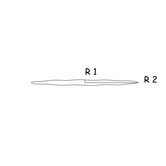
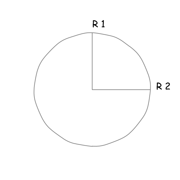
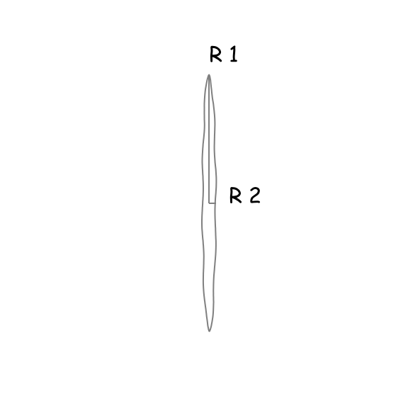
The Area of an Ellipse
Let’s use the method of easy cases to solve a simple problem: determine the area of an ellipse.
We know that an ellipse is this peculiar, circle-like object with two focal points, hence two radii. We can be pretty confident that the area of the ellipse will depend on those two radii and since their ratio is a dimensionless quantity, we can use it as our \(\beta\). Let’s investigate the behaviour of \(\beta\) for three regimes:
| Regime 1 | Regime 2 | Regime 3 |
|---|---|---|
| \(\frac{r_{1}}{r_{2}} =\beta \ll 1\) | \(\frac{r_{1}}{r_{2}} =\beta \approx 1\) | \(\frac{r_{1}}{r_{2}} =\beta \gg 1\) |
 |
 |
 |
| The area of the ellipse tends to 0. | The ellipse becomes a radius with the area \(r_{1}^{2}\pi\) (or \(r_{2}^{2}\pi\) ). | The area of the ellipse tends to 0. |
Regime 2 suggests that \(r_{1}^{2}\pi\) or \(r_{2}^{2}\pi\) may be the answer, but we know that those are particular cases of an ellipse. On the other hand, regimes 1 and 3 suggest, that there is a symmetry in the problem. Perhaps, in the general equation we need to include both \(r_1\) and \(r_2\)? This implies that interchanging \(r_{1}\) and \(r_{2}\) shall have no effect on the area of the ellipse. Those two pieces of information suggest that the correct equation should be:
\[A=r_{1}r_{2}\pi\]Indeed, this equation is correct for all three regimes.
Clearing the Atmosphere
Many phenomena around us are the result of the physical state of equilibrium achieved by the nature. An example of such a system, which is governed by the natural balance, is our atmosphere. We know that there are forces acting on the atmosphere, but since it is (approximately) at rest, some physical equilibrium is present.
Let’s test the usefulness of easy-cases method to answer the following question:
What is the height of Earth’s atmosphere?
When we think about the height, we are interested in forces which act perpendicular to the surface of the earth. All the bodies on our planet are being pulled towards the Earth due to gravitation. Why is the atmosphere not collapsing - pulled all the way to the ground? This is due to the thermal energy of atmosphere’s molecules. In absence of gravity the air molecules would basically scatter towards the space.
So from the perspective of one “atmosphere molecule” there are two competing effects: gravity and thermal energy. Since both quantities are some form of energy, their ratio is a dimensionless quantity:
\[\beta = \frac{E_\text{gravity}}{E_\text{thermal}}=\frac{mgh}{k_{b}T}\]Let’s think about the behaviour of the system in terms of easy-cases regimes:
| Regime 1 | Regime 2 | Regime 3 |
|---|---|---|
| \(\beta \ll 1\) | \(\beta \approx 1\) | \(\beta \gg 1\) |
| The dispersion of the molecules is stronger than the gravity - atmosphere expanding. | State of equilibrium - the atmosphere remains stable. | The dispersion of the molecules is weaker than the gravity - atmosphere contracting. |
Nature is biased towards equilibria so we should use regime 2 to continue with our problem - computing the height of the atmosphere. Temperature of the atmosphere is about 300 Kelvins, mass of the atmosphere can be approximated as a mass of a nitrogen molecule (Earth’s atmosphere is mostly nitrogen) and gravitational acceleration and Boltzmann constant are known to us.
\[h = \frac{Tk_b}{mg} \approx \frac{300 \cdot 1.38 \cdot 10^{-23}}{4.65 \cdot 10^{-26}\cdot 9.81} \approx 9000\text{m}\]In reality Earth’s atmosphere stretches from the surface of the planet up to as far as 10,000 kilometres above (after that, the atmosphere blends into space).
Conclusion: When the going gets tough, the tough lower your standards. A correct solution works in all cases, including the easy cases. Therefore, look at the easy cases first. Often, we can completely solve a problem simply by understanding the easy cases.
Tool #8 Look for the Spring-like Behaviour
The ideal spring, which you may know from high-school physics, produces a restoring force proportional to the displacement from equilibrium and stores an energy proportional to the displacement squared.
\[\Delta E= F\Delta x = -k\Delta x \cdot \Delta x = k(\Delta x)^2\]We have already established, that the nature likes equilibria. If you swing a system out of balance, it usually wants to restore its initial stability. So yes, you’ve guessed it: many physical process “contain” a spring. Spring models are therefore very useful abstraction that can be used to speak about the connections between chemical bonds, trajectories of the planets or biomechanics of the human body. It is also useful in the material engineering.
Young’s Modulus as a Spring Constant
Most engineering students at some point encounter the quantity known as Young’s modulus. It is a fundamental property of every material, which describes its stiffness - how easily it bends or stretches. However it is not directly visible, how every material can be envisioned as a huge set of tiny springs and masses.
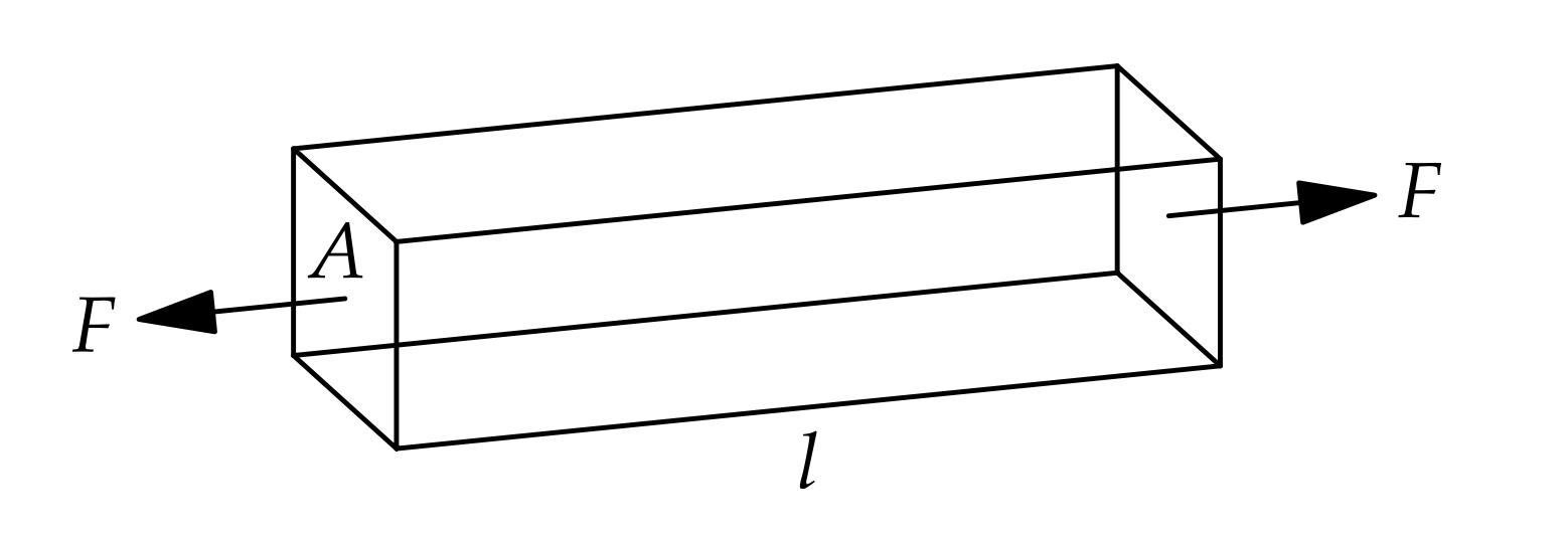
Image source: “The Art of Insight in Science and Engineering: Mastering Complexity”</div></div>
Young’s modulus is a function of two values: stress (the force applied to a material, divided by the its cross-sectional area) and strain (deformation of material that results from an applied stress).
\[Y = \frac{\text{stress}}{\text{strain}}\]While stress is straightforward to compute (using force applied and the cross-section of the block of material, \(\text{stress} = \frac{F}{A}\)), it can be quite difficult to compute material’s strain. However, we can easily estimate it through modelling a block of material as a system of springs and masses. Imagine that a block of material is in fact a bundle of tiny, elastic fibres.
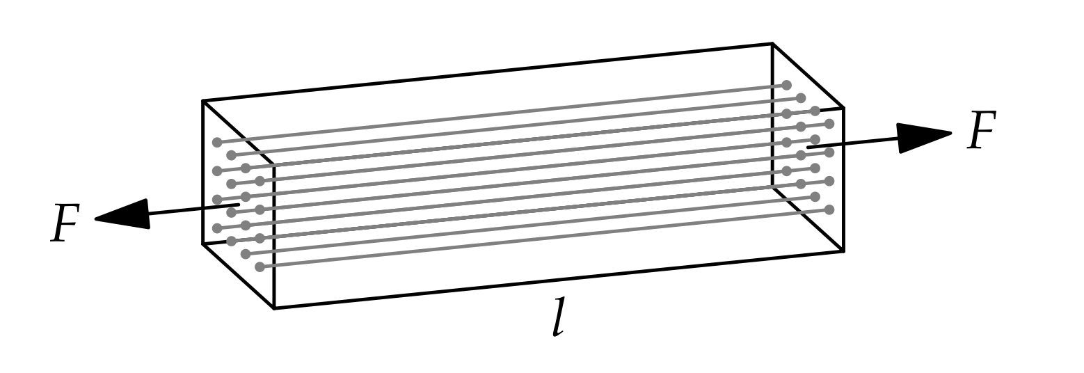
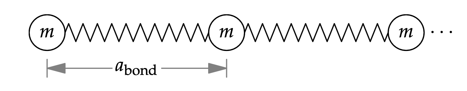
Each fibre is a chain (series) of springs (bonds) and masses (atoms).
Since strain is the fractional length change, the strain in the block is the strain in each fibre:
\[\text{strain} = \frac{\Delta x}{a}\]Where \(\Delta x\) is the extension of the spring and \(a\) is the length of the bond between two atoms at rest.
How to compute \(\Delta x\)? Using the spring equation for a single fibre:
\[\frac{F}{N_\text{fibres}} = k\Delta x\]Where \(F\) is the force acting on the block of material, \(N_\text{fibres}\) is the number of fibres in the block, \(k\) is the spring constant and \(\Delta x\) is the spring extension.
How many fibres are there in the block of materials? We know \(A\), the cross-section of the block of material. We also know the approximate cross-section of one fibre - \(a^2\), so:
\[N_\text{fibres} = \frac{A}{a^2}\]Notice, how we used divide-and-conquer reasoning to break down the problem into smaller components. Now let’s collect of the established information and derive the equation for Young’s modulus:
\[Y = \frac{\text{stress}}{\text{strain}} = \frac{\frac{F}{A}}{\frac{\Delta x}{a}}=\frac{Fa}{A\Delta x} = \frac{Fa}{A\frac{F}{kN_\text{fibres}}}= k\frac{aN_\text{fibres}}{A}=k\frac{a\frac{A}{a^2}}{A}=\frac{k}{a}\]So Young’s modulus has actually a neat micro-level interpretation. It a direct function of the interatomic spring constant \(k\) and the distance between atoms in the material’s lattice.
Conclusion: Many physical processes contain a minimum-energy state where small deviations from the minimum require an energy proportional to the square of the deviation. This behavior is the essential characteristic of a spring. A spring is therefore not only a physical object but a transferable abstraction.
Tool #7 Probabilistic Reasoning
The final element in our toolbox is probabilistic reasoning. Bayesian thinking is a very useful every-day “philosophy”- so it should come as no surprise, that we would like to include it in our back-of-the-envelope calculations. Probabilistic reasoning is a nice sprinkle on top of divide-and-conquer. It allows us to do the same decomposition of the problem as before, but now the estimated values are not point estimates anymore, they are probability distributions - confidence intervals.
Setzen Alles Auf Eine (Land-)Karte
Let’s estimate the area of Germany.
Method 1: Quick Order-of-Magnitude Estimation
To compute the area of a country, we can do quick order-of-magnitude estimation. Imagine that Germany has perfectly rectangular area. Given, that we speak in terms of kilometres, could the area of Germany be \(10 \times 10\)? Absolutely not! \(100 \times 100\)? Still, too little. \(1000 \times 1000\), probably too much… So it seems that the good estimate is somewhere between \(10^5\) and \(10^6\). I am pretty sure about that, so I may give 2-to-1 odds that the correct value lies in that range. 2-to-1 odds means that I attach probability \(P\approx 2/3\) to this statement.
.png)
Method 2: Divide-and-Conquer
This is the result obtained from rough estimation. Now let’s use divide-and-conquer reasoning. The rectangular area is product of two values: height and width.
The height of Germany is a bit more than a distance between Hamburg and Munich. Having spent a lot of time travelling between those cities in the past, I know that it takes about 8 hours by car to cross Germany north to south. This implies the distance of 1200 kilometres. While I am not sure about the exact value, I think that it’s not less than 800, but not more than 1500 kilometres. Once again, I attach probability of \(P\approx 2/3\) to this statement.
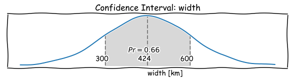
Germany is certainly longer than wider, so the width is less than the height. To travel from Berlin to the Dutch border it takes about 5 hours or so. I am not really sure, but I bet that it is not less than 300, and not more than 600 kilometres.
\[h_\text{divide-and-conquer} = 800...1500 \text{ }[\text{km}]\] \[w_\text{divide-and-conquer} = 300...600 \text{ }[\text{km}]\] \[A_{min, \text{divide-and-conquer}} = 800 \cdot 300 = 240,000 \text{ }[\text{km}]\] \[A_{max, \text{divide-and-conquer}} = 600 \cdot 1500 = 900,000 \text{ }[\text{km}]\].png)
We can already see the benefits of divide-and-conquer over the rough order-of-magnitude estimation - we are much more surer about the actual result. It has significantly narrowed the confidence interval by replacing a quantity about which we have vague knowledge (area), with quantities about which can be approximated much more precisely (width and height). The direct approximation gives us a range which spans over ratio of 10. However, divide-and-conquer gives the ratio of \(A_{max} / A_{min} \approx 3.75\).
Method 3: Divide-and-Conquer + Probabilistic Reasoning
We can express the estimation for height and width as probability distributions: log-normal distributions. There are three reasons for choosing this particular distribution: it is more compatible with our “mental hardware” (humans think in terms of ratios), easy to describe and simple to perform computations with. For example, confidence interval of the height can be characterised by a following (geometric) mean and standard distribution (ratio):
\[h_{\mu} = \sqrt{h_{min} \cdot h_{max}}=1095\] \[h_{\sigma} = \frac{h_{max}}{h_{\mu}} =\frac{h_{\mu}}{h_{min}} = 1.37\]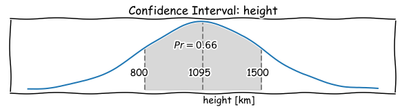
Same applies for the width.
Note, that one standard deviation, or one sigma, plotted above or below the average value on that normal distribution curve, elegantly defines a region that expresses (approximately) 2-to-1 odds.
Now to find the area, we can combine those two distributions, which is the “probabilistic” equivalent of multiplying two point estimates - width and height.
The mean is simply a product of geometric means:
\[A_{\mu} = h_{\mu} \cdot h_{\mu}= 464,758\text{ }[\text{km}^2]\]Standard deviation of product of two (independent) normal distributions is:
\[\sigma_{3} = \sqrt{\sigma_{1}^2 \cdot \sigma_{2}^2}\]However, in our log-normal form, the standard deviation of area needs to be computed in log space:
\[\ln\sigma_{A} = \ln(\sqrt{\sigma_{h}^2 + \sigma_{w}^2}) \implies \sigma_{A} = e^{(\sqrt{(\ln{\sigma_{h}})^2 + (\ln{\sigma_{w}})^2}}=1.60\]By combining divide-and-conquer with probabilistic reasoning we get the following estimate of the area:
\[A_{min, \text{probabilistic reasoning}} = A_{\mu} / A_{\sigma} = 291,094 \text{ }[\text{km}^2]\] \[A_{max, \text{probabilistic reasoning}} = A_{\mu} \cdot A_{\sigma} = 742,026 \text{ }[\text{km}^2]\] \[A_\text{probabilistic-reasoning} = 291, 094...742,026 \text{ }[\text{km}^2]\]…while the actual area of Germany is 357,386 square kilometres - comfortably included in my predicted range.
.png)
Probabilistic reasoning gives us the values range which spans only over the ratio of 2.55 (variance of the distribution).
How did we produce such accurate estimate? This problem is hard to analyse directly because we do not know the accuracy in advance. But we can analyse a related problem: how divide-and-conquer reasoning increases our confidence in an estimate or, more precisely, decreases our uncertainty.
Conclusion: In complex systems, the information is either overwhelming or not available. Then we have to reason with incomplete information. The tool for this purpose is probabilistic reasoning, which helps us manage incomplete information. It can e.g. help us to estimate the uncertainty in our divide-and-conquer reasoning.