Deep Dive into NeRF (Neural Radiance Fields)
I have to confess: recently I did not get to do a lot of horsing around with new, hot neural network architectures. I do not have as much time to fully reimplement papers as I used to as a university student. But luckily, I found out that if one has access to very good code, one can gain deep knowledge of an algorithm solely by running the code through my debugger, analyzing what is going on step-by-step, and cross-referencing ones understanding with the original paper. And plotting - a lot of plotting to visualize concepts; we humans are very visual beasts after all. So I set out to finally understand how this cool invention called NeRF (Neural Radiance Fields) works.
I was supposed to spend a rainy evening just clicking through the breakpoints in my debugger but ended up writing a pretty in-depth blog post. Oh well…
The code that I analyzed was the one by Krishna Murthy. I highly recommend his tinynerf implementation. Very well-written, clean, and thoroughly documented code.
Introduction
The goal of NERF is to render high-quality images conditioned on the pose of the observer (the camera). NeRF is an example of a neural rendering technique- we explicitly control one of the properties of the scene - the pose of the observer - to obtain rendered images corresponding to that pose. The model learns a continuous volumetric scene function, that can assign a color and volume density to any voxel in the space. The network’s weights are optimized to encode the representation of the scene so that the model can easily render novel views seen from any point in space.
Think about it as “distilling” or “compressing” the information about some 3D space, like your apartment for instance, into a very tiny set of parameters (the parameters of NeRF).
Below, I will explain step-by-step how that is being done.
Step 1: Marching the Camera Rays Through the Scene
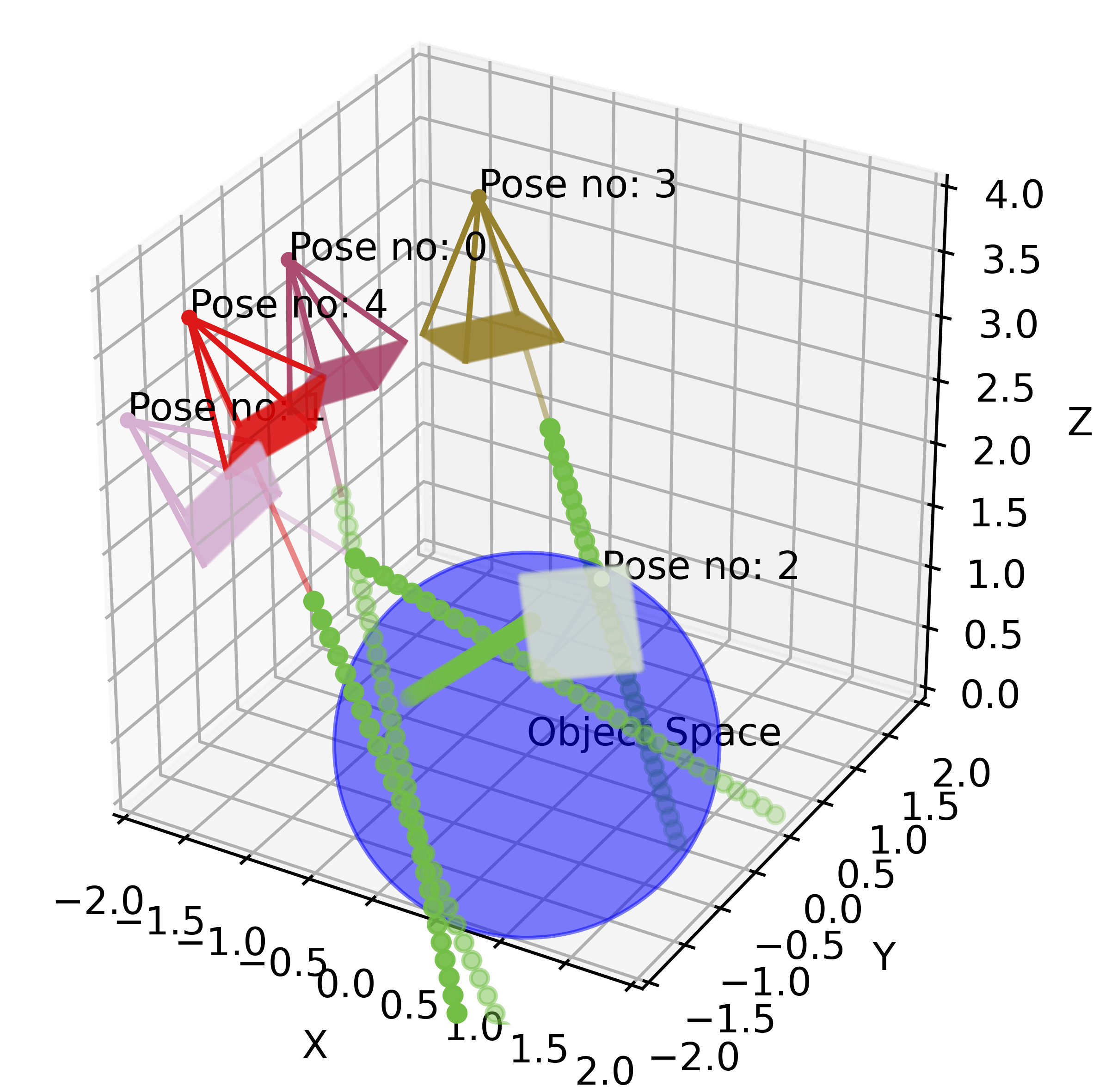
Input: A set of camera poses \(\{x_c, y_c, z_c, \gamma_c, \theta_c\}_n\)
Output: A bundle of rays for every pose \(\{\mathbf{v_o}, \mathbf{v_d}\}_{H\times W\times n}\)
Let’s look at the problem setup. The object that we want to render is located in the point \((0,0,0)\) (world coordinates). The object is placed in a 3D scene, which we will call the object space. A camera is fixed in the space at the position \((x_c, y_c, z_c)\). Since the camera is always “aimed” at the object, we only need two more rotation parameters to fully describe the pose: the inclination and azimuth angles \((\gamma_c, \theta_c)\). In the dataset, we have \(n\) pairs of poses, together with the corresponding ground truth images.
In front of the camera, we place the image plane. Intuitively, the image plane is our “canvas”, this is where all the 3D information from the rays will be aggregated to render a 2D image (3D to 2D projection). The size of the image plane is \(H\times W\).
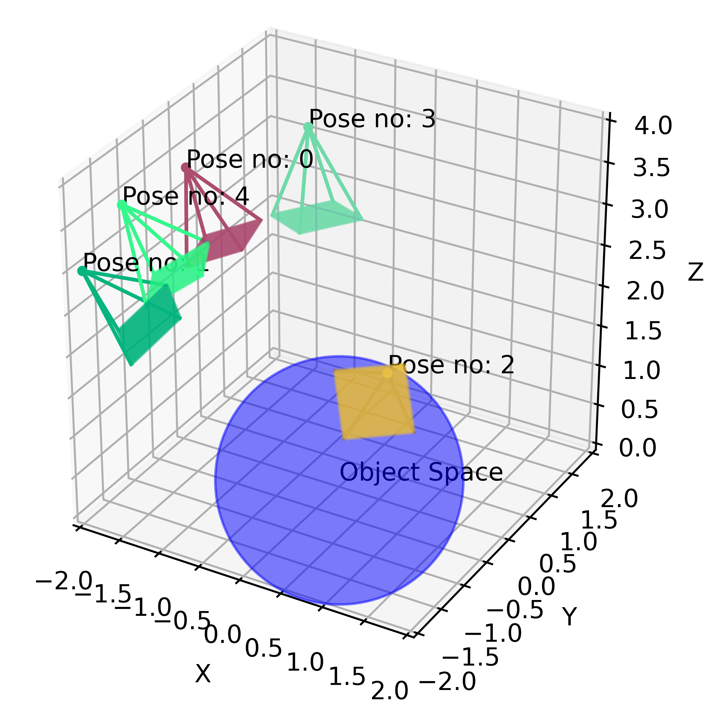
Now, we “shoot” a bundle of rays from the camera, through every pixel of the image plane, resulting in \(H \times W\) rays per pose.
Every ray is described by two vectors:
- \(\mathbf{v_o}\), a vector that specifies the origin of the ray. Note that \(\mathbf{v_o} = (x_o, y_o, z_o) = (x_c, y_c, z_c)\)
- \(\mathbf{v_d}\), a normalized vector that specifies the direction of the ray.
Parametric equation \(P = \mathbf{v_o} + t * \mathbf{v_d}\) defines any point on the ray. So to do the “ray marching”, we make the \(t\) parameter larger (thus extending our rays) until a ray reaches some interesting location in the object space.
This type of ray-tracing process described above is called backward tracing. This is because we follow the path of light rays from the camera to the object, rather than from the light source to the object.
If you’d like to learn more about ray tracing in general, I highly recommend one of the courses from the great Scratchapixel website: Rendering an Image of a 3D Scene: an Overview.
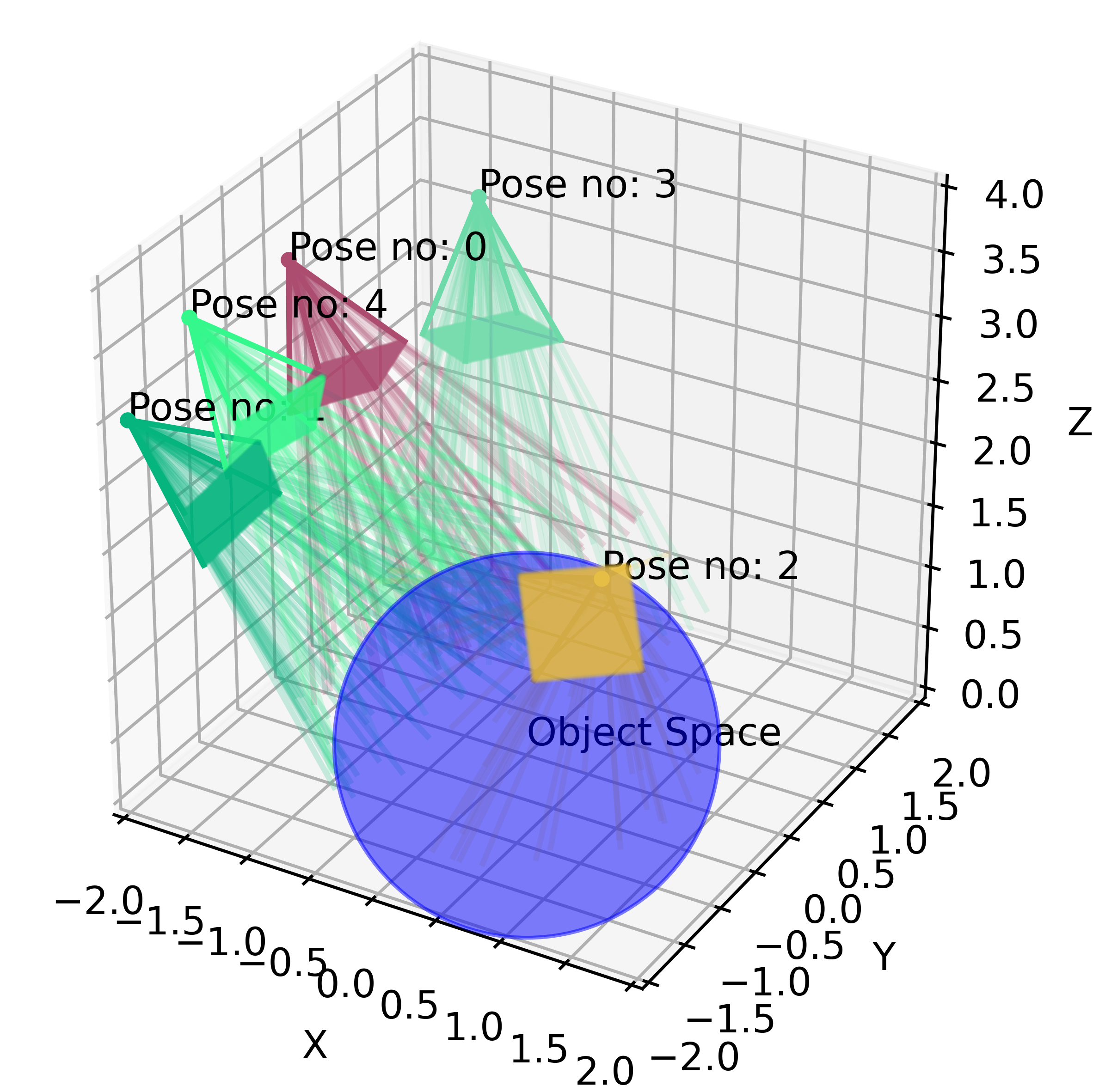
Step 2: Collecting Query Points
Input: A bundle of rays for every pose \(\{\mathbf{v_o}, \mathbf{v_d}\}_{H\times W\times n}\)
Output: A set of 3D query points \(\{x_p, y_p, z_p\}_{n\times m \times H \times W}\)
In computer graphics, the 3D scene is very often modeled as a set of tiny, discrete region “cubes” called voxels. When a ray “flies” through the scene, it will pass through a large number of points in space. Most of those points represent “emptiness”, however, some may land on the object volume itself. The latter points are very valuable to us - they give us some knowledge about the scene. To render an image we will query the trained neural network, whether a point, some tiny piece of scene volume, belongs to the object or not, and more importantly, which visual properties it has. We can intuitively see that sampling points along a ray is not trivial. If we sample a lot of points that do not belong to the object space we won’t get any useful information. Still, if we only sample some high-volume density regions (points around the mode of the volume density distribution), we may miss out on some other interesting areas.
In our toy example, we sample uniformly along the ray (for every ray we sample \(m\) points). But for better performance, authors use “hierarchical volume sampling” to allocate samples proportionally to their expected effect on the final rendering. For more details, refer to the original paper.
Step 3: Projecting Query Points to High-Dimensional Space (Positional Encoding)
Input: A set of 3D query points \(\{x_p, y_p, z_p\}_{n\times m \times H \times W}\)
Output: A set of query points embedded into \(d\)-dimensional space \(\{x_{1}, x_2, ... ,x_d\}_{n\times m \times H \times W}\)
Once we collect the query points for every ray, we are potentially ready to feed them into the neural network. However, the authors of the paper argue, that before the inference step, it is beneficial to map the query points to a high-dimensional space. The mapping is very particular - it uses a set of high-frequency functions.
It is a well-known fact, that neural networks (after all - universal function approximators) are much better at approximating low-frequency, rather than high-frequency functions:
[…] we highlight a learning bias of deep networks towards low-frequency functions – i.e. functions that vary globally without local fluctuations – which manifests itself as a frequency-dependent learning speed. Intuitively, this property is in line with the observation that over-parameterized networks prioritize learning simple patterns that generalize across data samples.
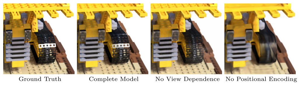
This observation is very important in the context of NeRF. The high-frequency features, such as colors, detailed geometry, and texture, make images perceptually sharp and vivid for the human eye. If our network is unable to represent those properties, the resulting image may look bleak or over-smoothed. However, the way the network improves over time is similar to watching an object emerge from the fog. First, we see a general silhouette, its coarse outline, and dominant colors. Only later we might notice details, texture, and more fine-grained elements of an object.
The authors claim that mapping the inputs to a higher dimensional space using high-frequency functions before passing them to the network enables better fitting of data that contains high-frequency variation. In our example, we use two functions - sine and cosine - to embed the points in high-dimensional space.
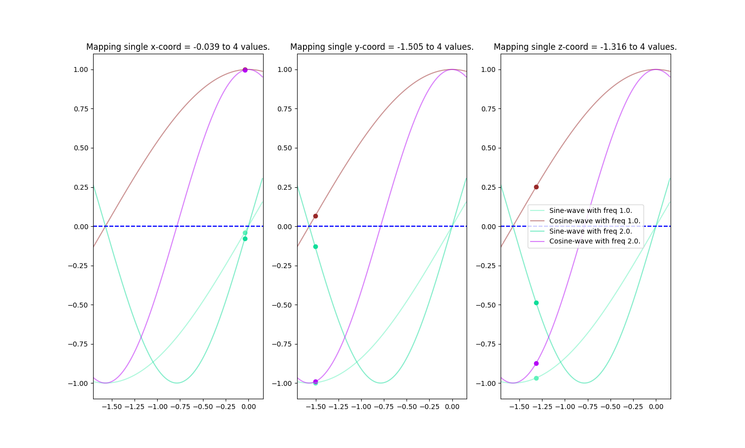
The image above is a graphical representation of a mapping of a random point \(p=[-0.039, -1.505, -1.316]\) using an encoding function \(\gamma(p)\):
\[\gamma(p) = (\sin(\pi p), \cos(\pi p), \sin(2\pi p), \cos(2\pi p)) = ([-0.039, -0.998, -0.968], [0.999, 0.065, 0.251], [-0.079, -0.123, -0.486], [0.997, -0.992, -0.874])\]Step 4: Neural Network Inference and Volume Rendering
Neural Network Inference
Input A set of 3D query points (after positional encoding) \(\{x_{1}, x_2, ... ,x_d\}_{n\times m \times H \times W}\)
Output RGB colour and volume density for every query point \(\{RGB, \sigma\}_{n\times m \times H \times W}\)
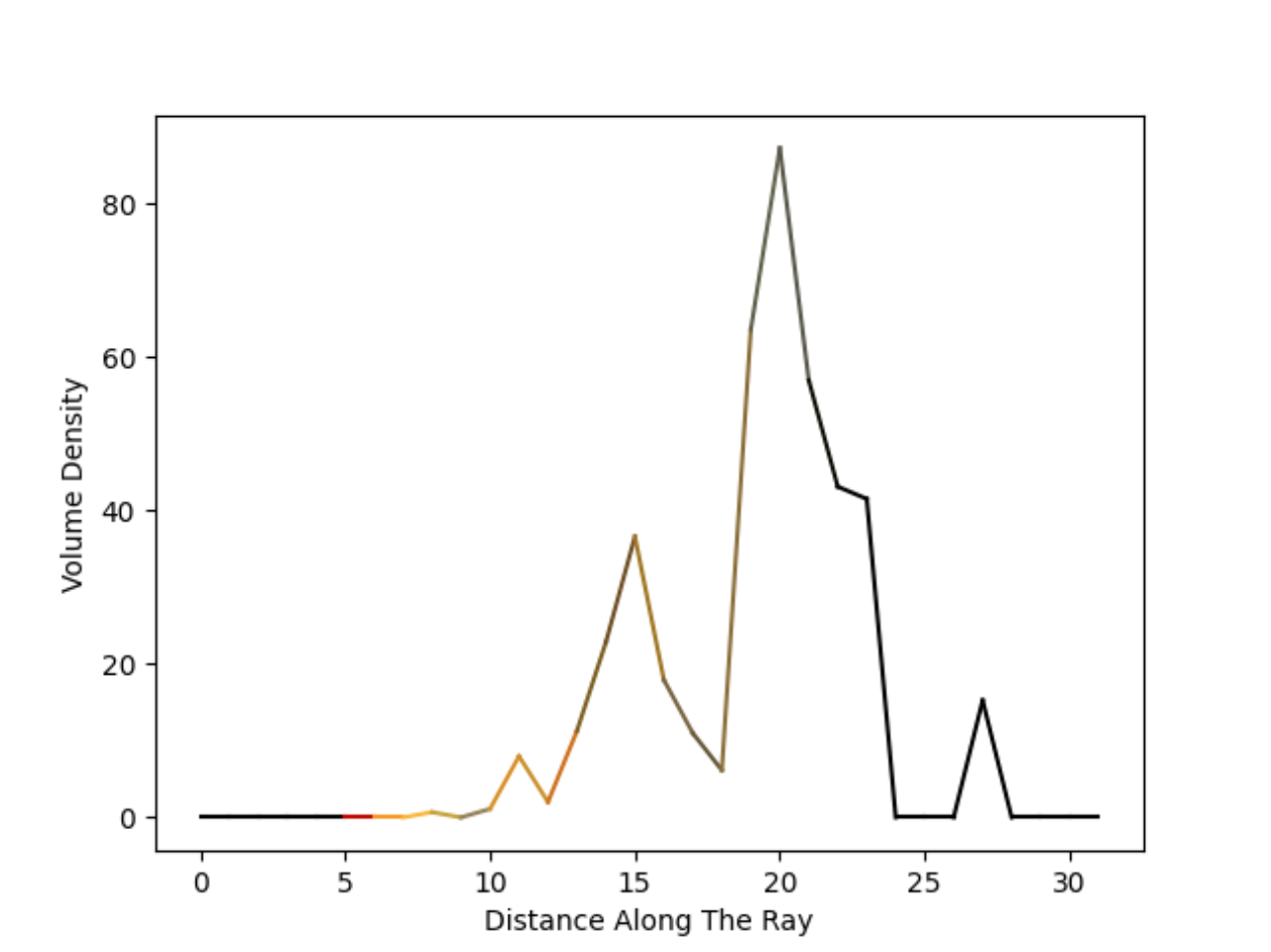
We feed the representation of query points into the NeRF network. The network returns the RGB value (tuple of three values in the range from 0 to 1) and volume density (a single, positive integer) for every point. This allows us to compute the volume density profile for every ray.
Volume Rendering
Input A set of 3D query points (after positional encoding) + their volume profile + RGB value \(\{x_{1}, x_2, ... ,x_d, RGB, \sigma\}_{n\times m \times H \times W}\)
Output A set of rendered images (one per pose) \(\{H,W\}_{n}\)
Next, we may turn the volume density profile along a ray into a pixel value. Then we repeat the process for every pixel in the image and voila, we have just rendered the image.
To aggregate the information from all the points along a single ray, we use the classical equation from computer graphics, the rendering equation. It is an integral equation in which the equilibrium radiance leaving a point is given as the sum of emitted plus reflected radiance under a geometric optics approximation.
In the context of NeRF, because we use straight rays and approximate the integral using samples, this seemingly perplexing integral can be simplified to a very elegant sum.
We compute a sum of all the RGB values from all the points along the ray, weighted by the probability of the ray stopping at any given point when flying from the observer into the scene (see equation \(3\) from the original paper). The higher the volume density of the point, the higher the probability of the ray stopping at that point, and thus the probability that the RGB value of that point will have a significant impact on the final RGB file of the rendered pixel.
Once again, I recommend reading more about volume rendering on Scratchapixel website.
Computing the Loss
Input A set of rendered images (one per pose) \(\{H,W\}_{n}\) and a set of ground truth images (one per pose) \(\{H,W\}^{gt}_{n}\)
Output L2 loss between the inputs, a single scalar \(\{l\}_{n}\)
Finally, we compute the loss by comparing the pixels of the rendered image with the pixels of the ground truth image. Then we backpropagate this loss to optimize the weights of the network.
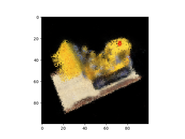
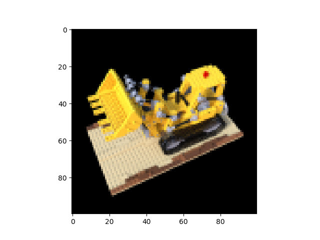
As a bonus, attaching a gif generated while I was playing with the code.