
Tutorial - Visual Attention for Action Recognition
Action recognition is the task of inferring various actions from video clips. This feels like a natural extension of image classification task to multiple frames. The final decision on the class membership is being made by fusing the information from all the processed frames. Reasoning about a video remains a challenging task because of high computational cost (it takes more resources to processes three-dimensional data structures than 2D tensors), difficulty of capturing spatio-temporal context across frames (especially problematic when the position of a camera changes rapidly) or the difficulty of obtaining a useful, specialized dataset (it is much easier and cheaper to collect vast amounts of independent images then image sequences).
Independently of the action recognition problem, the machine learning community observed a surge of scientific work which uses soft attention model - introduced initially for machine translation by Bahdanau et. al 20141 . It has gotten more attention then its sibling, hard attention, because of its deterministic behavior and simplicity. The intuition behind the attention mechanism can be easily explained using human perception. Our visual processing system tends to focus selectively on parts of the receptive field while ignoring other irrelevant information. This helps us to filter out noise and effectively reason about the surrounding world. Similarly, in several problems involving language, speech or vision, some parts of the input can be more relevant compared to others. For instance, in translation and summarization tasks, only certain words in the input sequence may be relevant for predicting the next word.
The purpose of this blog post is to present how the visual attention can be used for action recognition. I will give a short overview of the history, discuss the neural network architectures used in the tutorial together with the implementation details and finally present the results produced by two methods: Attention LSTM (ALSTM) and Convolutional Attention LSTM (ConvALSTM). The implementation described in this tutorial can be found in my github repo.
Table of Contents
- Short Historical Background
- Attention LSTM for Action Recognition
- Making Attention LSTM Fully Convolutional
- Implementation Details, Results and Evaluation
- References
- Footnotes
Short Historical Background
The surge of deep learning research in the domain of action recognition came around year 2014. That’s when the problem has been successfully tackled from two angles. Karpathy et al. 2014 2 used convolutional neural networks (CNNs) to extract information from consecutive video frames and then fused those representations to reason about the class of the whole sequence. Soon Simmoyan and Zisserman 2014 3 came up with different solution - a network which analyzes two input streams independently: one stream reasons about the spatial context (video frames) while the second uses temporal information (extracted optical flow). Finally both pieces of information are combined so the network can compute class score. Another work introduced by Du Tran et al. 20144 uses 3D convolutional kernels on spatiotemporal cube. Lastly, one of the most popular approaches was proposed by Donahue et al. 2014 5 . Here, the encoder-decoder architecture takes each single frame of the sequence, encodes it using a CNN and feeds its representation to an Long-Short Term Memory (LSTM) block. This way we “compress” the image using feature extractor and then learn the temporal dependencies between frames using recurrent neural network.
With the increasing popularity of attention mechanisms applied to the tasks such as image captioning or machine translation, incorporating visual attention in the action recognition tasks became an interesting research idea. The work by Sharma et al. 20166 may serve as an example. This is the first method which will be covered in this article. This idea has been improved by Z.Li et al. 2018 7 where three further concepts were introduced. Firstly, the spatial layout of the input is being preserved throughout the whole network. This was not the case in the previous approach, where image was flattened at some point and treated as a vector. Secondly, the authors additionally feed optical flow information to the network. This makes the architecture more sensitive to the motion between the frames. Finally, the attention is also being used for action localization. This work will also be partially covered in this tutorial. For the sake of completeness it is important to mention that visual attention was also combined with 3D CNNs by Yao et al. 2015 8 . It is pretty fascinating how this concept has been successfully applied some many different domains and methods!
Attention LSTM for Action Recognition
Summary of the Method
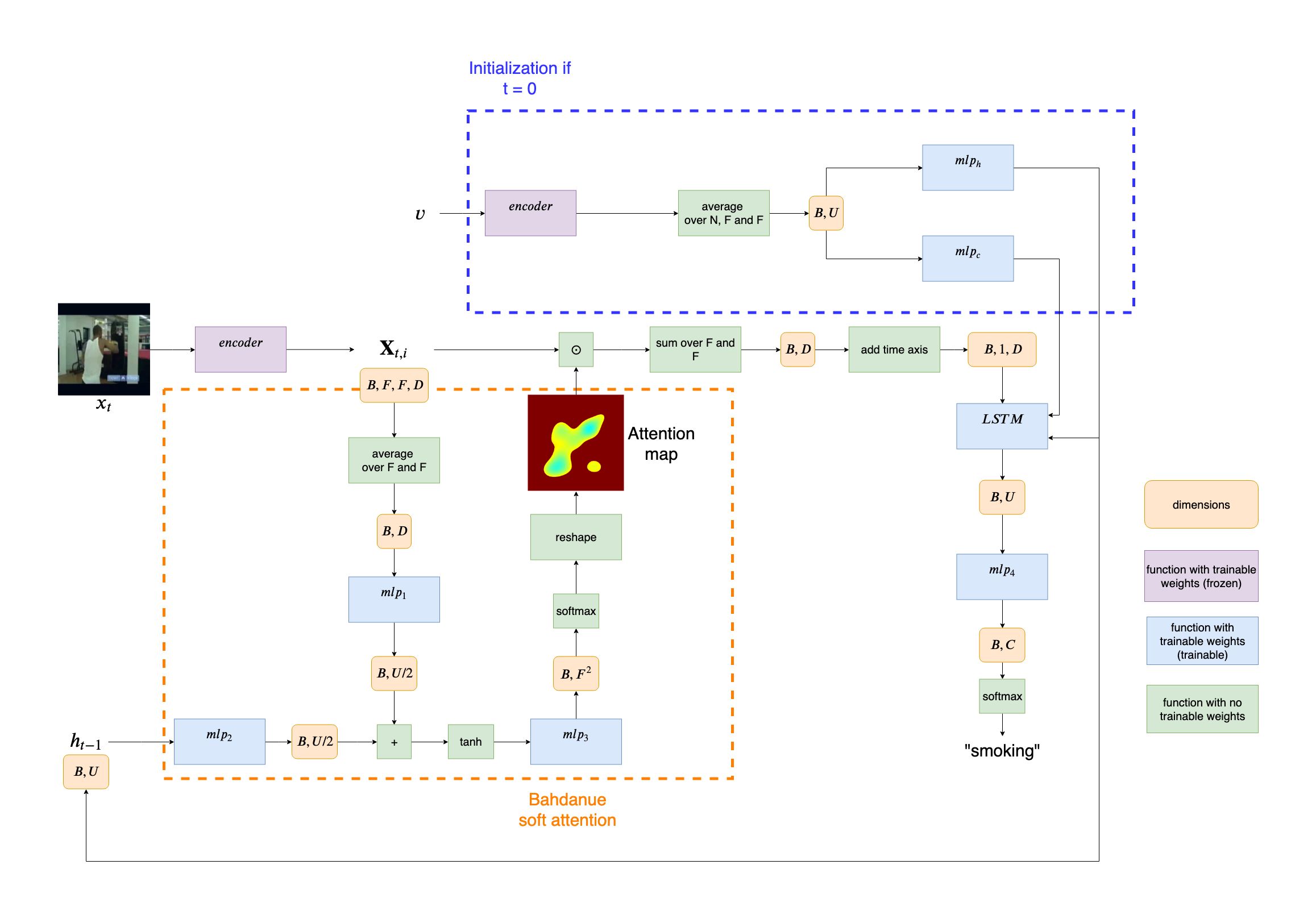
In the work by Sharma et al., the problem of video classification has been tackled in the following manner. Let’s denote a video \(v\) as a set of images, such that \(v = \{x_1, x_2, ..., x_T\}\). Every sequence consists of $30$ frames. The appearance of individual video frame \(x_t\) is encoded as a feature cube (a feature map tensor) \({\mathbf{X}_{t,i}} \in \mathbb{R}^{D}\) derived from the last convolutional layer of a GoogLeNet. In our implementation we will use much simpler feature extractor - VGG network - thus the feature cubes have shape \(7\times7\times512\). So in our particular implementation:
\[t \in \{1,2,...,30\}\] \[i \in \{1,2,...,7^2\}\] \[D=512\]Then, the model combines the feature cube \({\mathbf{X}}_{t,i}\) with the respective attention map \(c_{t}\in \mathbb{R}^{F^2}\) (how we get those maps - I will explain soon) and propagates its vectorized form through an LSTM. The recurrent block then outputs a “context vector” \(h_t\). This vector is being used not only to predict the action class of the current frame but is also being passed as a “history of the past frames” to generate next attention map \(c_{t+1}\) for the frame \(x_{t+1}\).
Let’s take a closer look the the network. It can be dissected into three components:
Soft attention block
This element of the network is responsible for the computation of the attention map \(c_t\). That is done by compressing a feature cube into a vector form (averaging over the dimensions \(F,F\) for every channel of a feature cube) and finally creating a mapping from the “context vector” \(h_{t-1}\) and current compressed frame vector to a score vector \(s_t\):
\[s_t = mlp_{3}(tanh(mlp_{1}(\frac{1}{F^2}\sum_{i=1}^{F^2}{\bf{X}}_{t,i})+mlp_{2}(h_{t-1})))\]In order to produce the final attention map, we need to additionally apply softmax to the generated vector \(s_t\) and reshape the representation so it matches a 2D grid. This way we obtain a \(F\times{F}\) tensor, a probability distribution over all the feature map pixels. The higher the value of the pixel in the attention map, the more important this image patch is for the classifier’s decision
Final classification of weighted feature cube
First, we multiply element-wise each feature map in \(\mathbf{X}_{t,i}\) with the obtained attention map \(c_t\). The resulting input has the same shape as \(\mathbf{X}_{t,i}\). Now for every channel we sum up all the pixels of a feature map and end up with a single vector in \(\mathbb{R}^{D}\). In order to feed this representation to the LSTM we need to insert a time dimension. Finally the output from the LSTM, \(h_{t}\) is being used in two ways. On one hand it is processed by fully connected layer to reason about the class of \(x_{t}\). On the other hand it is being passed on to serve as a “context vector” for \(x_{t+1}\).
LSTM hidden state and cell state initialization
Drawing inspiration from Xu et al. 2015 , this approach uses the compressed information about the whole video \(v\) to initialize \(h_{0}\) and \(c_{0}\) for faster convergence.
\[h_0 = mlp_h(\frac{1}{T}\sum_{t=1}^{T}(\frac{1}{F^2}\sum_{i=1}^{F^2}{\mathbf{X}_{t,i}}))\] \[c_0 = mlp_c(\frac{1}{T}\sum_{t=1}^{T}(\frac{1}{F^2}\sum_{i=1}^{F^2}{\mathbf{X}_{t,i}}))\]We pass all the frames in \(v\) through an encoder network which produces \(T\) feature cubes. In order to compress this representation we take an average first over the number of feature cubes and then over all pixel values in each feature map. Resulting vector is being finally into two multi-layered-perceptrons: \(mlp_h\) (which produces \(h_{0}\), the “zeroth” context vector for \(x_{1}\)) and \(mlp_c\) (which outputs \(c_{0}\), the initial cell state of the LSTM layer).
Making Attention LSTM Fully Convolutional
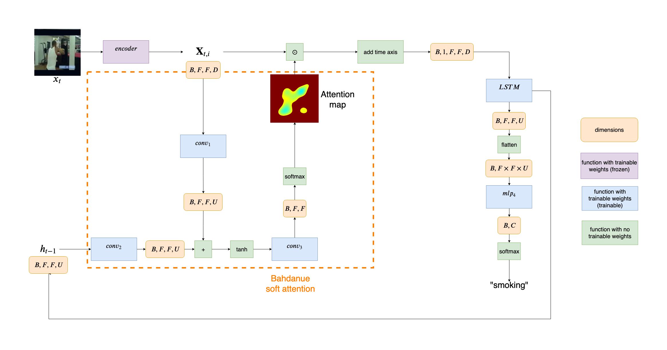
As mentioned before, the work Z. Li et al. introduces three new ideas regarding visual attention in action recognition. For the purpose of this tutorial I will focus only on the first concept, which is adapting the soft-attention model in such a way, that the spatial structure is preserved over time. This means introducing several changes to the current architecture:
- Removing the cell state and hidden state initialization block. While the authors of ALSTM did follow the initialization strategy for faster convergence, it seems that the network does fine without this component. This means that we only need to initialize the hidden state as a tensor of zeros every time the first frame of the given video enters the pipeline.
- Keeping the network (almost) entirely convolutional. Treating images as an 2D grid rather then a vector helps to preserve a spatial correlation (in this regard the convolutions are much better then inner products), leverages local receptive field and allows weight sharing. Therefore we substitute all fully connected layers for convolutional kernels (except for the last classification layer) and use convolutional LSTM instead of the standard one. Thus the hidden state is not a vector anymore, but a 3-D tensor.
Implementation Details, Results and Evaluation
HMDB-51 Dataset Processing
This dataset is composed of 6766 videoclips from various sources and has 51 action classes.
For the purpose of my implementation, for every video in the dataset I extract every second frame, thus reducing the sampling rate from the original 30fps to 15fps. Then I split each video into multiple groups of 30 frames. I follow the first train/test split proposed by the authors of the dataset, so in the end I use 3570 videos for training, 1130 for validation and 400 for testing.
Implementation details
It takes just few epochs for both ALSTM and ConvALSTM to converge. For regularization I use dropout in all fully connected layers, early stopping and weight decay. The results are satisfying, but there are still many improvements possible e.g. performing a thorough hyper-parameter tuning (time consuming process which I have decided to skip). I think that the model would especially benefit from the optimal numbers of units in dense layers (ALSTM) or kernels in convolutional layers (ConvALSTM), as well as number of LSTM/ConvALSTM cells. Finally, the output to the ConvALSTM is a tensor of size \(F \times F \times U\). Before it is consumed by fully connected layer it needs to be flattened. The resulting size of the vector is quite large. It would be a good idea to feed it to some convolutional layers first before using the fully connected network.
The ALSTM contains an additional component in its loss, the attention regularization (Xu et al. 2015). This forces the model to look at each region of the frame at some point in time, so that:
\[\sum_{t=1}^{T}c_{t,i}\approx 1 \space where \space c_t = \frac{e^{s_{t,i}}}{\sum_{j=1}^{K^2} e^{s_{t,j}}}\]The regularization \(\lambda\) term decides whether the model explores different gaze locations or not. I have found out that \(\lambda=0.5\) is adequate for my ALSTM.
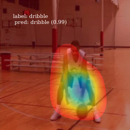
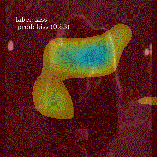
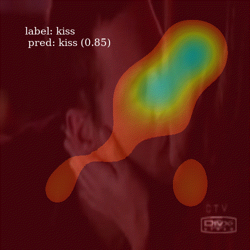
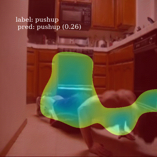
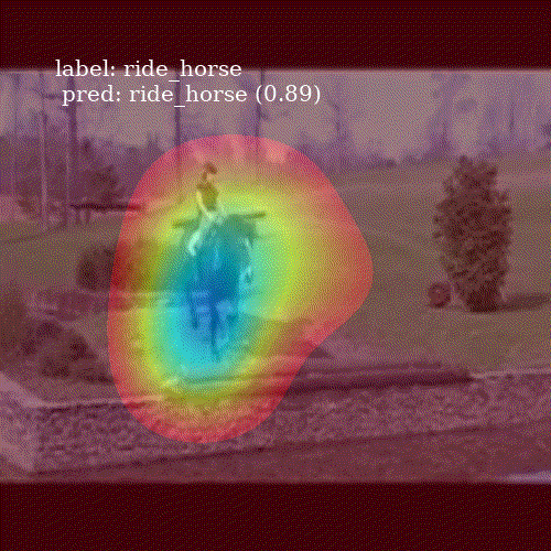
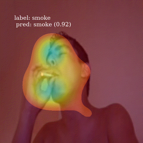
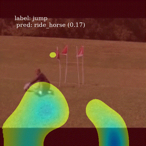
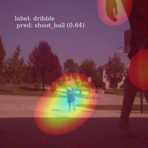
To visualize an attention map \(c_i\), I take its representation, a \(7 \times 7\) matrix, and upsample to \(800 \times 800\) grid. I smooth it using Gaussian filter and keep only those values higher then the \(80^{th}\) percentile of the image pixels. This removes noise from the heatmap and allows to clearly inspect which parts of the frame were important for the network.
| Symbol | Description | ALSTM | ConvALSTM |
|---|---|---|---|
| B | batch size | 16 | 16 |
| F | dimension of the feature map extracted from VGG’s pool5 layer | 7 | 7 |
| D | number of feature maps extracted from VGG’s pool5 layer | 512 | 512 |
| U | number of LSTM units (ALSTM) or number of channels in the convolutional kernel of convolutional LSTM (ConvALSTM) | 512 | 256 |
| C | number of classes | 51 | 51 |
| \(dt\) | dropout value at all fully connected layers | 0.5 | 0.5 |
| \(\lambda\) | attention regularization term | 0.5 | \(-\) |
| \(\omega\) | weight decay parameter | 0 | \(-\) |
| \(-\) | accuracy of the model (test set) | \(56.0\)% | \(52.5\)% |
Description of models’ parameters
Results
It is interesting to see how well the network attends to meaningful patches of a video frame. Even though ALSTM achieves higher accuracy then ConvALSTM, the latter does much better job when it comes to attention heatmap generation. To obtain a prediction for an entire video clip, I compute the mode of predictions from all 30 frames in the video.
Successful predictions
ALSTM
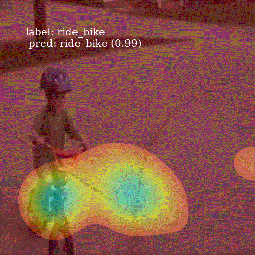

ConvALSTM
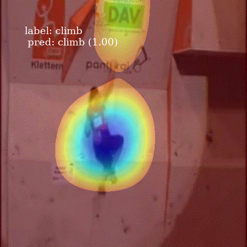
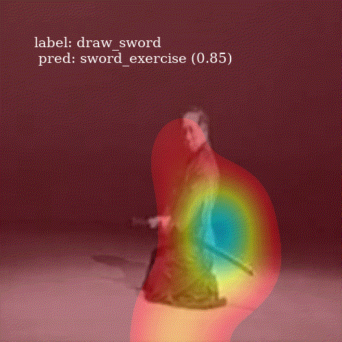
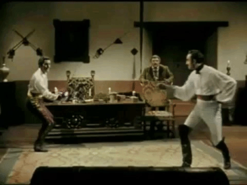
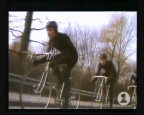
Failure cases
ALSTM

ConvALSTM

References
In the article I have used information from review of action recognition
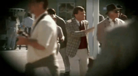
Source of the cover image: www.deccanchronicle.com